
Data Structure
E N D
Presentation Transcript
Data Structure Chapter 3 Visit for more Learning Resources
Searching Searching is a process of finding out a particular element in a list of ‘n’ elements
Methods of Searching • Linear Search (Sequential Search) • Binary Search
Linear Search(Sequential Search) In a linear search, we start at the top of the list, and compare the element there with the key If we have a match, the search terminates and the index number is returned
Linear Search Comparison = 05
Linear Search No of Comparisons = 11
Binary Search • A binary search is a divide and conquer algorithm In a binary search, we look for the key in the middle of the list If we get a match, the search is over If the key is greater than the thing in the middle of the list, we search the top half If the key is smaller, we search the bottom half
Binary Search Beg = 0 End = 6 Mid = 0+6/2 Search Element = 25 If(key==a[mid] 0 1 2 3 4 5 6 6 13 14 25 33 43 51
Binary Search Beg = 0 End = 6 Mid = 0+6/2 Search Element = 13 0 1 2 3 4 5 6 6 13 14 25 33 43 51 If 13 < a[mid] then search in the left side. Beg = 0 End = mid – 1 Mid = 0+2/2
Binary Search Beg = 0 End = 6 Mid = 0+6/2 0 1 2 3 4 5 6 6 13 14 25 33 43 51 If key > a[mid] Beg = mid+1 End = 6 Mid = 4+6/2
Difference between linear and binary search • Linear Search 1. Data can be in any order. 2. Multidimensional array also can be used. 3.TimeComplexity:- O( n) 4. Not an efficient method to be used if there is a large list. • Binary Search • Data should be in a sorted order. • Only single dimensional array is used. • Time Complexity:- O(log n 2) • Efficient for large inputs also.
Sorting (Bubble Sort) 5 4 4 4 4 4 5 3 3 3 3 3 5 2 2 2 2 2 5 1 1 5 1 1 1 1 2 3 4 5
77 11 33 2 6 1 99 77 11 33 2 6 1 99 1 11 33 2 6 77 99 1 2 33 11 6 77 99 77 , 11 , 33 , 2 , 6 , 1 , 99
1 2 6 11 33 77 99 1 2 6 11 33 77 99 1 2 6 11 33 77 99
Insertion Sort 1. Insertion sort keeps making the left side of the array sorted until the whole array is sorted. It sorts the values seen far away and repeatedly inserts unseen values in the array into the left sorted array. 2. It is the simplest of all sorting algorithms. Although it has the same complexity as Bubble Sort, the insertion sort is a little over twice as efficient as the bubble sort.
77 11 33 2 6 1 99 -99 77 -99 11 77 -99 11 33 77 -99 2 11 33 77 -99 2 6 11 33 77 -99 1 2 6 11 33 77 -99 1 2 6 11 33 77 99
Quick Sort Given an array of n elements (e.g., integers): • If array only contains one element, return • Else • pick one element to use as pivot. • Partition elements into two sub-arrays: • Elements less than or equal to pivot • Elements greater than pivot • Quicksort two sub-arrays • Return results
Example of Quick Sort 40 20 10 80 60 50 7 30 100 • Choose an element as the pivot element. • Given a pivot, partition the elements of the array such • that the resulting array consists of: • 1. One sub-array that contains elements >= pivot • 2. Another sub-array that contains elements < pivot
Example 40 20 10 80 60 50 7 30 100 30 20 10 80 60 50 7 40 100 30 20 10 40 60 50 7 80 100 30 20 10 7 60 50 40 80 100
30 20 10 7 40 50 60 80 100 30 20 10 7 40 50 60 80 100 Subpart 1 Subpart 2 30 20 10 7 50 60 80 100 7 20 10 30 Subpart 4 Subpart 3
60 80 100 7 20 10 Subpart 5 20 10 10 20 Sorted Elements 7 10 20 30 40 50 60 80 100
Algorithm of Quick Sort • //Sort an array A of n elements. • Create global integer array A[1:n+1]; • //The elements to be sorted are in A[1]…….A[n] • //Step 1: Put a very large element in A[n+1]; • //Find maximum of the n elements. • //Store a large element at the end of the sequence in A. • void max(1,n) • { • int max; • max = A[1]; • for (int I=2; I<=n; I++}
if (max < A[I]) max = A[I]; • A[n+1] = ++max; • return(0); • } • //The Quicksort algorithm • void Quicksort(int left, int right) • { • if (left >= right) return(0); • int pivot = Partition(left, right + 1); • Quicksort(left, pivot – 1); • Quicksort(pivot + 1,right); • return(0); • }
//Partititon returns position of the pivot element • //The pivot element is assumes to be the leftmost one • int Partititon(int left, int right) • { • int pivot_element = A[left]; • int left_to_right = ++left; • int right_to_left = --right; • while(A[left_to_right] < pivot_element) ++left_to_right; • while(A[right_to_left] > pivot_element) ++right_to_left; • //posititon for pivot element is at right_to_left • A[left] = A[right_to_left], A[right_to_left] = pivot_element; • return (right_to_left); • }
Merge Sort • Merge-sort is a sorting algorithm based on the divide-and-conquer paradigm . • Divide: divide the input data S in two disjoint subsets S1and S2 • Recur: solve the subproblems associated with S1and S2 • Conquer: combine the solutions for S1and S2 into a solution for S
40 20 10 80 60 50 7 30 20 40 10 80 50 60 7 30 10 20 40 80 7 30 50 60 7 10 20 30 40 50 60 80
Algorithm for Merge Sort • MERGE (A, R, LBA, S, LBB, C, LBC) • Set NA:= LBA, NB := LBB, PTR := LBC, UBA:= LBA+R-1, UBB := LBB+S-1. • Return. • MERGEPASS (A, N, L, B) • Set Q: = INT(N/(2*L)), S := 2*L*Q and R := N-S. • Repeat for J= 1, 2, ....,Q:a) Set LB: = 1+(2*J-2)*L. • b) Call MERGE(A, L, LB, A, L, LB+L, B, LB) • [End of loop]
3. If R<=L, then:Repeat for J=1, 2... R: • Set B(S+J) := A(S+J) • [End of loop] • Else: • Call MERGE(A, L, S+1, A, R, L+S+1, B, S+1) • Return
MERGESORT (A, N) • Set L := 1. • Repeat Steps 3 to 6 while L<N: • Call MERGEPASS(A, N, L, B) • Call MERGEPASS(B, N, 2*L, A) • Set L := 4*L[End of step 2 loop] • Exit
Radix Sort • Sorted Elements • 12 , 45 , 121
Shell Sort • Founded by Donald Shell and named the sorting algorithm after himself in 1959. • 1st algorithm to break the quadratic time barrier but few years later, a sub quadratic time bound was proven • Shellsort works by comparing elements that are distant rather than adjacent elements in an array or list where adjacent elements are compared.
Shell Sort • Shellsort makes multiple passes through a list and sorts a number of equally sized sets using the insertion sort.
Shell Sort • Sort: 18 32 12 5 38 33 16 2 • D1 = n/2 (8/2 = 4) • 18 16 12 5 38 33 32 2
2 32 12 5 38 33 16 18 D2 = d1/2 (4/2 = 2)
Shell Sort Advantage • Advantage of Shellsort is that its only efficient for medium size lists. For bigger lists, the algorithm is not the best choice. Fastest of all O(N^2) sorting algorithms. • 5 times faster than the bubble sort and a little over twice as fast as the insertion sort, its closest competitor. For more detail contact us