Stability Margins
Stability Margins. Professor Walter W. Olson Department of Mechanical, Industrial and Manufacturing Engineering University of Toledo. Outline of Today’s Lecture. Review Open Loop System Nyquist Plot Simple Nyquist Theorem Nyquist Gain Scaling Conditional Stability

Stability Margins
E N D
Presentation Transcript
Stability Margins Professor Walter W. Olson Department of Mechanical, Industrial and Manufacturing Engineering University of Toledo
Outline of Today’s Lecture • Review • Open Loop System • Nyquist Plot • Simple Nyquist Theorem • Nyquist Gain Scaling • Conditional Stability • Full NyquistTheorem • Is stability enough? • Margins from Nyquist Plots • Margins from Bode Plot • Non Minimum Phase Systems
Loop Nomenclature Disturbance/Noise Reference Input R(s) Error signal E(s) Output y(s) Controller C(s) Plant G(s) Prefilter F(s) Open Loop Signal B(s) Sensor H(s) + + - - The plant is that which is to be controlled with transfer function G(s) The prefilter and the controller define the control laws of the system. The open loop signal is the signal that results from the actions of the prefilter, the controller, the plant and the sensor and has the transfer function F(s)C(s)G(s)H(s) The closed loop signal is the output of the system and has the transfer function
Note: Your book uses L(s) rather than B(s) To avoid confusion with the Laplace transform, I will use B(s) Open Loop System Error signal E(s) Output y(s) Input r(s) Controller C(s) Plant P(s) Open Loop Signal B(s) Sensor -1 + +
Simple Nyquist Theorem Error signal E(s) Output y(s) Input r(s) Imaginary Controller C(s) Plant P(s) -B(iw) Plane of the Open Loop Transfer Function Open Loop Signal B(s) -1 is called the critical point -1 B(0) Sensor -1 Real Stable B(iw) Unstable + + Simple Nyquist Theorem: For the loop transfer function, B(iw), if B(iw) has no poles in the right hand side, expect for simple poles on the imaginary axis, then the system is stable if there are no encirclements of the critical point -1.
Nyquist Gain Scaling • The form of the Nyquist plot is scaled by the system gain
Conditional Stabilty • Whlie most system increase stability by decreasing gain, some can be stabilized by increasing gain • Show with Sisotool
Definition of Stable • A system described the solution (the response) is stable if that system’s response stay arbitrarily near some value, a, for all of time greater than some value, tf.
Full Nyquist Theorem • Assume that the transfer function B(iw) with P poles has been plotted as a Nyquist plot. Let N be the number of clockwise encirclements of -1 by B(iw) minus the counterclockwise encirclements of -1 by B(iw)Then the closed loop system has Z=N+P poles in the right half plane.
Is Stability Enough? • If not Why Not?
Margins • Margins are the range from the current system design to the edge of instability. We will determine • Gain Margin • How much can gain be increased? • Formally: the smallest multiple amount the gain can be increased before the closed loop response is unstable. • Phase Margin • How much further can the phase be shifted? • Formally: the smallest amount the phase can be increased before the closed loop response is unstable. • Stability Margin • How far is the the system from the critical point?
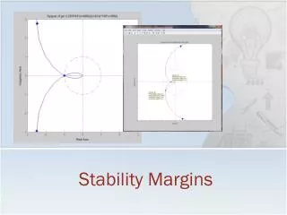
Example Using Matlab command nyquist(gs)
Example Here the gain from the previous plot has been multiplied by 3.2359 The result is that stability is about to be lost
Example Using Matlab command nyquist(gs)
Gain and Phase Margin DefinitionBode Plots Magnitude, dB 0 Positive Gain Margin w Phase, deg -180 Phase Margin w Phase Crossover Frequency
Example Using Matlab command bode(gs)
Example Again, stability is about to be lost.
Example Using Matlab command bode(gs)
Note • The book does not plot the Magnitude of the Bode Plot in decibels. • Therefore, you will get different results than the book where decibels are required. • Matlab uses decibels where needed.
Stability Margin • It is possible for a system to have relatively large gain and phase margins, yet be relatively unstable. Stability margin, sm
Non-Minimum Phase Systems • Non minimum phase systems are those systems which have poles on the right hand side of the plane: they have positive real parts. • This terminology comes from a phase shift with sinusoidal inputs • Consider the transfer functions • The magnitude plots of a Bode diagram are exactly the same but the phase has a major difference:
Another Non Minimum Phase SystemA Delay • Delays are modeled by the function which multiplies the T.F.
Summary • Is stability enough? • Margins from Nyquist Plots • Margins from Bode Plot • Non Minimum Phase Systems Next Class: PID Controls