Introduction to potential theory – at black board Potentials of simple spherical systems

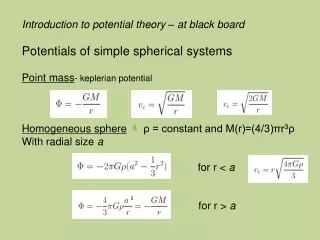
1. Introduction to potential theory – at black board Potentials of simple spherical systems Point mass- keplerian potential Homogeneous sphere ρ = constant and M(r)=(4/3)πr3ρ With radial size a for r < a for r > a 3

2. Isochrone potential – model a galaxy as a constant density at the center with density decreasing at larger radii. One potential with these properties: where b is characteristic radius that defines how the density decreases with r Density pair given in BT (2-34) and yields at center and at r >>b Modified Hubble profile – derived from SBs for ellipticals where a is core radius and j is luminosity density

3. Power-law density profile – many galaxies have surface brightness profiles that approximate a power-law over large radii If we can compute M(r) and Vc(r) If α = 2, this is an isothermal sphere (density goes as 1/r2)  Can be used to approximate galaxies with flat rotation curves; need outer cut-off to obtain finite mass

4. Plummer Sphere – simple model for round galaxies/clusters This potential “softens” force between particles in N-body simulations by avoiding the singularity of the Newtonian potential. The density profile has finite core density but falls as r-5 at large r (too steep for most galaxies). Jaffe and Hernquist profiles Both decline as r-4 at large radii which works well with galaxy models produced from violent relaxation (i.e. stellar systems relax quickly from initial state to quasi-equilibrium). Hernquist has gentle power-law cusp at small r while Jaffe has steeper cusp. Potential density

5. Density distributions for various simple spherical potentials

6. Navarro, Frenk and White (NFW) profile Good fit to dark matter halos formed in simulations Problem – mass diverges logarithmically with r  must be cut off at large r Potentials for Flattened Models: Axisymmetric potential Kuzmin Disk (cylindrical coordinates) At points with z<0, Φk is identical with the potential of a point mass M at (R,z) = (0,a) and when z>0, Φk is the same as the potential generated by a point mass at (0,-a). Everywhere except on plane z=0

7. Use divergence theorem to find the surface density generated by Kuzmin potential Kuzmin (1956) or Toomre model 1 (1962) Miyamoto & Nagai (1975) introduced a combination Plummer sphere/Kuzmin disk model where b is aP in previous Plummer notation a=0  Plummer sphere b=0  Kuzmin disk b/a ~ 0.2 similar to disk galaxies

8. Stellar Orbits • For a star moving through a galaxy, assume its motion does not change the overall potential • If the galaxy is not collapsing, colliding, etc., assume potential does not change with time • Then, as a star moves with velocity v, the potential at its location changes as • Recall (grad of potential is force on star) • Then, • Energy along orbit remains constant (KE always + ; PE goes to 0 at large x) • Star escapes galaxy if E > 0 • Circular velocity angular velocity

9. In a cluster of stars, motions of the stars can cause the potential to change with time. The energy of each individual star is no longer conserved, only the total for the cluster as a whole. cluster KE cluster PE Stars in a cluster can change their KE and PE as long as the sum remains constant. As they move further apart, PE increases and their speeds must drop so that the KE can decrease.

10. The virial theorem tells how, on average, KE and PE are in balance Begin with Newton’s law of gravity and add an external force F Take the scalar product with xα and sum over all stars to get… VT is tool for finding masses of star clusters and galaxies where the orbits are not necessarily circular. For system in steady-state (not colliding, etc), use VT to estimate mass Assume average motions are isotropic <v2> ≈ 3σr2 KE ≈ (3σr2/2) (M/L) Ltot Get PE by M = Ltot (M/L) then use galaxy SB to find volume density of stars.

11. Orbits in Spherical Potentials – at blackboard Equations of motion: In n spatial dimensions, some orbits can be decomposed into n independent periodic motions – regular orbits Integrals of Motion – functions of phase-space coordinates that are constant along any orbit (not time dependent) Regular orbits have n isolating integrals and define a surface of 2n-1 dimensions 2 independent integrals of motion are:

12. Each integral of motion defines a surface in 3-d space (R, VR, Vϕ) Constant E surface revolves around R-axis Constant L surface is a hyperbola in the R, Vϕ plane Intersection is closed curve and the orbit travels around this curve Vϕ VR R *note that both L and J are used to denote angular momentum The integrals of motion combine (see BT 3.1 for treatment) to produce a differential equation where u = 1/R

13. Solutions to this equation have 2 forms: bound = orbits oscillate between finite limits in R unbound = R  ∞ or u  0 Each bound orbit is associated with a periodic solution to this equation. Star in this orbit also has a periodic azimuthal motion as it orbits potential center. Relationship between azimuthal and radial periods is: is usually not a rational number so orbit is not closed in most spherical potentials • star never returns to starting point in phase-space • typical orbit is a rosette and eventually passes every point in annulus between pericenter and apocenter

14. Two special potentials where all bound orbits are closed • Keplerian potential – point mass • - radial and azimuthal periods are equal • - all stars advance in azimuth by between successive pericenters • 2) Harmonic potential – homogeneous sphere • - radial period is ½ azimuthal period • - stars advance in azimuth by between successive pericenters • Real galaxies are somewhere between the two, so most orbits are rosettes advancing by •  Stars oscillate from apocenter to pericenter and back in a shorter time than is required for one complete azimuthal cycle about center

15. Orbits in Axisymmetric Potentials – at blackboard Φeff = ½ Vo2 ln (R2 + z2/q2) + Lz2/(2R2) Φ(R,z) • q= axial ratio • Resembles Φ of star in oblate spheroid with constant Vc = Vo • Φeff rises steeply toward z-axis

16. If only E and Lz constrain motion of star on R,z plane, star should travel everywhere within closed contour of constant Φeff • But, stars launched with different initial conditions with same Φeff follow distinct orbits • Implies 3rd isolating integral of motion – no analytically form

17. Nearly Circular Orbits in Axisymmetric Potentials – epicyclic approximation In disk galaxies, many stars are on nearly circular orbits derive approximate valid solutions to d2R/dt2 and d2z/dt2. Taylor expansion series around (Rg,0) or (x,z) = (0,0) (Ignore higher order terms) Note: x = R – Rg  yields harmonic potential Define two new quantities: Epicyclic and Vertical frequencies Then equations of motion become x and z evolve like the displacements of 2 harmonic oscillators with frequency κ and ν

18. Integrals of Motion are then Now relate back to the potential…recall Then the equations become Since the angular speed is related to the potential as We can now write kappa in terms of the angular speed This is related to the (well known) Oort constant B

19. The Oort constants, first derived by Jan Oort in 1927, characterize the angular velocity of the Galactic disk near the Sun using observationally determined quantities. • It can be shown that • Ωo = A – B • κ2 = -4B(A-B) = -4BΩo at the Sun • Hipparchos proper motions of nearby stars yield (Feast & Whitlock 1997): • A = 14.8 ± 0.8 km/s/kpc • B = -12.4 ± 0.6 km/s/kpc • κo = 36 ± 10 km/s/kpc • Sun makes 1.3 oscillations in radial direction in the time to complete one orbit around GC • Does not close (rosette) A measures “shear” in the disk – would be zero for solid body rotation B measures rotation of Galaxy or local L gradient

20. Continue with Nearly Circular orbit approximation on the board…. Integrals of motion Equations of motion in x , z and y directions Derive epicycle shapes X/Y = κ/(2Ω) Pt mass (keplarian rotation curve) κ=Ω and X/Y=1/2 Homogeneous sphere κ=2Ω and X/Y=1

21. Orbits in Non-Axisymmetric Potentials • Produce a richer variety of orbits – Φ = Φ (x,y) or Φ (x,y,z) cartesian coordinates • Only 1 classical integral of motion – E = ½ v2 + Φ • though other integrals of motion may exist for certain potentials which cannot be represented in analytical form • Orbits in non-axisymmetric potential can be grouped into Orbit Families. Examples can be found in two types of NAPs. • Separable Potentials • All orbits are regular (i.e. the orbits can be decomposed into 2 or 3 independent period motions (in 2 or 3-d) • All integrals of motion can be written analytically • These are mathematically special and therefore not likely to describe real galaxies. However, numerical simulations for NA galaxy models with central cores have many similarities with separable potentials. • Distinct families are associated with a set of closed, stable orbits. In 2-d: • Oscillates back and forth along major axis (box orbits) • Loops around the center (loop orbits)

22. 2-D orbits in non-axisymmetric potential • For larger R > Rc, orbits are mostly loop orbits • initial tangential velocity of star determines width of elliptical annulus (similar to way in which width of annulus in AP varies with Lz) • Rotation curve is flat with q=1 at large R • For small R<<Rc, orbits become box orbits • potential approximates that of homogeneous sphere • orbits are like harmonic oscillator

23. Triaxial potentials with cores have orbit families like those in separable potentials. In 3-d (triaxial potential), there are four families of orbits: box orbit: move along longest (major) axis, parent of family short axis tube orbit: loop around minor axis (resemble annular orbit of axisymmetric potential Intermediate and short axis orbits are unstable! inner long-axis tube orbit: loop around major axis outer long-axis tube orbit: loop around major axis Intermediate axis loop orbits are unstable!

24. Scale Free Potentials • All properties have either a power-law or logarithmic dependence on radius (i.e. ρ ~ r-2) • These density distributions are similar to central regions of E’s and halos of galaxies in general • If density falls as r-2 or faster, box orbits are replaced by boxlets • box orbits about minor-axis arising from resonance between motion in x and y directions (Miralda-Escude & Schwarzchild 1989) • Some irregular orbits exist as well (i.e. stochastic motions which wander anywhere permitted by conservation of energy).

25. Stellar Dynamical Systems • Unlike molecules in a gas, where collisions distribute and average out their motions, stellar systems are governed strictly by gravitation forces. • For stars, the cumulative effect of small pulls of distant stars is more important than large pulls caused as one star passes close to another. But we will see that even these have little effect over a galaxy’s lifetime of randomizing or relaxing the stellar motions. Therefore, • The smooth Galactic potential of the Milky Way almost entirely dominates the motion of the Sun. • Consider a system where physical collision are rare. This can be idealized as N point-sized bodies with masses Mi, positions ri and velocities vi Potential runs over all pairs twice, hence the 1/2 Equations of motion are

26. A general result of the equations of motions is the scalar virial theorem where T is KE and U is PE since E = T + U Total mass M and energy E of N-body system define a characteristic velocity and size  the virial velocity and virial radius The crossing time is a system can be then be defined tc is constant even for systems far from equilibrium tc is time scale over which system evolves toward equilibrium

27. For systems near equilibrium, Vv2 = GM/Rv density For systems w/galaxy-like profiles Rv = 2.5 Rh (half-mass radius) tc ~ 1.36 (Gρh)-0.5 where density is defined within the half-mass radius Since crossing time is supposed to be just the typical time scale for orbital motion, we can define the crossing time as Under virial assumptions, crossing time depends only on density and increases as density decreases to the square power. How does the crossing time relate to the relaxation time, or time it would take the small pulls of distant stars to randomize the stellar orbits? tc = (Gρh)-0.5

28. In a distant encounter, the force of one star on another is so weak that stars hardly deviate. We can use the impulse approximation to calculate the forces that a star would feel as it moves along an undisturbed path ΔVt where ΔVt = 2Gm/(bV) m impact parameter But, when is it a close enough encounter to matter?? A strong encounter occurs when, at closest approach, the change in the PE is as great as the initial KE Gm2/r ≥ 1/2mV2 so r ≤ rs = 2Gm/V2this is the strong encounter radius Near the Sun, V ~ 30 km/s, m ~ 0.5 M then, rs ~ 1 AU  pretty close! How often does this occur? Assume the Sun is moving with speed V for a time t through a cylinder with radius rsand volume π rs2 V t. What is time ts such that n π rs2 V t = 1? = 1015 yrs with typical solar values

29. Back to considering effects of distant encounters… Using impulse approximation, a star will have dnenc encounters during a single passage through a system area of annulus with radius b and width db Surface density of stars The star receives many deflections due to dn encounters, each with random direction, so expected tangential velocity after time t is obtained by adding perturbations in quadrature Each decade between bmin and Rv contribute equally to total deflection Note: rs=2bmin Total velocity perturbation acquired in one crossing time So a single distant encounter may barely effect the star, but the cumulative effects are important!

30. Now estimate V as the virial velocity Vv where Vv ~ sqrt(GNm/Rv) and let Then… ….is the total change in a star’s velocity per crossing time tc Relaxation time is the time over which the cumulative effects of stellar encounters become comparable to a star’s initial velocity For galaxies N~1011 stars and tr = 5x108 tc (relaxation important after ~100 million crossings) But, galaxies in general are only ~100 crossing times old  cumulative effects of encounters between stars are pretty insignificant! For globular clusters, N~106 or 105 stars and tc~105 yrs tr=5000tc stellar encounters important after ~109-1010 yrs In denser cores, encounters play a key role…

31. Collisionless Dynamics – In the continuum limit, stars move in the smooth gravitational field Φ(x,t) of the galaxy. So instead of thinking about motion in 6N dimensions, we can simplify to just 6 dimensions. Galaxy may be described by a one-body distribution function (probability density in phase-space): f(x,v,t)ΔxΔyΔzΔvxΔvyΔvz -average number of stars in phase-space volume at (x,v) and time t Number density (at position x) is then n(x,t) = integral f(x,v,t) d3v Average velocity <v(x,t)>n(x,t) = integral v f(x,v,t) d3v Find equations relating changes in the density and DF to the gravitational potential as stars move about the galaxy…

32. As stars move through a galaxy, how do changes in the density and DF of stars relate to the potential? vx • Simplify to one direction x • n(x,t) Δx is # stars in “box” between x and x+Δx at time t • After time Δt: x x+Δx Δx[n(x,t + Δt) – n(x,t)] = n(x,t)v(x) Δt – n(x+Δx,t) v(x+Δx) Δt entered in Δt left in Δt Left side is the change in # between the two times and right side is change in stars entering and leaving which should be equivalent

33. Take limits at Δt  0 and Δx  0 Equation of continuity – stars are not destroyed or added Rate of stars flowing in + rate of stars flowing out is zero. The Collisionless Boltzmann equation is like the EOC, but allows for changes in velocity and relates changes in DF to forces on the stars. • Assume acceleration of star dv/dt depends only on potential at (x,t) • If dv/dt>0, after Δt all stars will be moving faster by Δt(dv/dt) • Stars with velocities between v and • v-Δt(dv/dt) move in • Those with velocities below v+Δv have left (x+Δx,v+Δv) v + Δv v (x,v) x x+Δx Then, the net # of stars gained the center box after Δt due to change in v and x

34. In the limit that all Δ’s are small EOC in phase-space space Under gravity, stars’ acceleration depends only on position So, I-D CBE And in 3D Collisionless Boltzmann Equation – the fundamental equation of stellar dynamics

35. Equation holds if stars are neither created or destroyed and change position & velocity smoothly. BT describe CBE this way = “The flow of stellar phase points through phase space is incompressible; the phase-space density f around the phase point of a given star always remains the same.” If there are close encounters between stars, these can alter the position and velocity much faster than a smoothed potential. In this case, the effects are given as an extra “collisional” term on the right side. Since f is a function of seven variables (phase-space and time), the complete solution of CBE is usually too difficult – but, velocity moments of CBE can be used to answer specific questions in stellar dynamics

36. Integrate CBE over velocity and apply  0th velocity moment  1st velocity moment where i=1-3 (3D) 1. 0th moment of CBE This is the EOC – no surprise since we just integrate over velocity Now multiply CBE by vj and integrate over velocity and apply  2nd velocity moment 2. 1st moment of CBE

37. From 2nd moment of velocity, velocity dispersion is Combine 1 and 2 and divide by n 3. 2 acceleration kinematic viscosity gravity pressure -analogous to Euler’s equation in fluid mechanics Equations 1, 2, and 3 are known as Jeans Equations (Sir James Jeans, 1919) - first applied to stellar dynamics

38. 2 • Applying Jeans Equations and CBE – Mass Density in the Galactic Disk • Select tracer stellar type (K dwarfs) and measure density n(z) at height z above disk (coordinates (z, vz) instead of (x, v)) • Assume potential, DF and number density n do not change with time • At large z, <vz>n(z)  0, thus Eq. 1 gives <vz> = 0 everywhere • Eq. 3 with σ = σz and since <vz>=0 we lose the 1st and 2nd term If we measure how density and sigma changes with z, we get vertical force at any height z. Now use Poisson’s Eq., which relates that force to mass density of the Galaxy. Assume MW is axisymmetric so potential and density only depend on R, z This is equal to Vc2(R)

39. Since V(R) is ~constant at Sun, let the last term = 0 Then, if we know # density wrt z and the velocity dispersion in z, we get density! More accurate to determine mass surface density Σ than volume density ρ Oort (1932) measured n(z) for F dwarfs and K giants and obtained Σ (<700pc)=90 Msun/pc2 (assumed σz didn’t vary with height) ρo(Ro,0)=0.15 Msun/pc3 Bahcall (1984) gets ρo(Ro,0)=0.18 Msun/pc3 averaging several tracers

40. More recent work with fainter K dwarfs (more numerous and evenly spread out) indicates σz increases with z: • σz ~ 20 km/s @ 250 pc and 30 km/s @ 1 kpc • Yields Σ (<1100pc) = 71 +/- 6 Msun/pc2 • If some of this is in the halo, disk is ~50 to 60 Msun/pc2 • Compare this dynamical estimate to mass summed up in gas and stars in the disk  40 to 55 Msun/pc2 • Not much DM in the disk What is disk surface density required to maintain a flat rotation curve? Σrot = Vc2/(2πGRo) ~ 210 Msun/pc2 - way too big!! Also tells us that most of this mass must be distributed in a halo component well out of the disk (scale height above 1 kpc)