Calibration, error modeling and variance stabilization of microarray data
Calibration, error modeling and variance stabilization of microarray data. Anja von Heydebreck Martin Vingron MPI Molecular Genetics Berlin. Wolfgang Huber Holger Sültmann Annemarie Poustka Div.Molecular Genome Analysis DKFZ Heidelberg. Overview IAM, Univ. HD, 13 Feb 2003.

Calibration, error modeling and variance stabilization of microarray data
E N D
Presentation Transcript
Calibration, error modeling and variance stabilization ofmicroarray data Anja von HeydebreckMartin Vingron MPI Molecular Genetics Berlin Wolfgang HuberHolger Sültmann Annemarie Poustka Div.Molecular Genome Analysis DKFZ Heidelberg
OverviewIAM, Univ. HD, 13 Feb 2003 o What are microarrays good for? - functional genomics - cancer o What do they measure? (very schematically) o The data and the challenges o Model formulation o Simplification by variance stabilizing transformation o Parameter estimation o Results simulated data real data
But what does the sequence do? >gi|22046029|ref|NT_029998.5|Hs7_30253 Homo sapiens chromosome 7 reference genomic contig GATCTTATCTATCATGTTCACCTCCCAAGAGGTGAACATATCCCCCAAAGCCTGATAGAGAGAAGATGCTCATTAATATTTAATGCATGACCATGTGCAGACTTGGGAGGAAAAATATGCCTCAGCCTATCAATATTGGACCTTAATAAACAAGGATGTTTCTGCATCATTTCCCCACAACACCGAACAAGTGTGGCTCACTGTGGATGTTTAAGCAAATGCATTGTTTTTCCAGTTATATATCTGGTAGAGATGAGGCCATTGATAGGAATGGGAAGACGATCTCCTTTTATTTTGATGACCCAGCATGGCTGAACACTCAGTGACTACCACTGCACTTTGTTGTACTTTCAGCATTAGAGATGCCAGCCCTGTAGGATATAAAACAGGAACATCTAGTCCTCAATTATATTCAGAATTACTCAAGTCTTAGAAGCACCACTTGTCTTTTTTCAAGGGAGAGAAATGCTCAAGTGATGGGCTGAAGTGAAGGGAGGGAGTCACTCACTTGAACGGTTCCCTTAGGCTGTGTGGATGCAAACAGCATTAGACAATGACACTGACAGTGGGAAATGCACTGGAGACGATGACTGGCAAAGCCCTCCTTTTCTCCCCATCCACTATAGATACTGACAGCAAAGGGTTTGTCACAATGACAACTATACACTCCCAATATCACAGAAGAAGGAGGAATAAAAGGGTATATTATGAGTGACTGAAGTTTAGAATAAATTAATAAATATTATGTCCCTCATCCATAGAAACCACAAAGGTCTAGTAAGGCTAAGGATATAACAAGAAAATAATATGAATATTTGCTTCCCCTTCCTAGTGTAATAGAGTAAGTTACAAATGGCTTCAGGAAGGGGAGAGAGGAAGAAGAGTGGATGAGATACGTAAGAGTGCTTGAGGGCTAATTTTATGAAAGCTTTGGGAAGTTTTAAGAAAAAGAAAAGCTATTTTTCAAGGTACATGTGTGTATGCGTGTGTGTGTGTGTGTGTGTGTGTGTGTGTGTGTGTGTGTGTGAAAGACAGAAGAAAGAGGGAGACCTAAGAAGACTATGAGACACTAAGAGAAAAATTAAGGTAAAAAAGACACACACTTAGAAAAACACACATAGGGAGGAGGGAGGAGGTTAAGACATTTTACTATGTGCTGTGAATGGAAACTACAAACCATTTTTGATATATGCAATATATATACATATATACACACATATACATATGTATTTAAATATTTAAATTACATTTTCTCTTTTTTTAGAGATATGGTTTCACTATGTCACTCTGCCCAGGCTGCAGTACAGTGGTTGTTCACAGTCATGATCATAGCACATTATAGCCTTGAACTCCTGGGCTCAAGCAACCCTCCTGTATTAGTCTCCCCAGTAGTTGGGATTACTAGCATATGCCACCATGTCCACCTTTATGCTTTTTAAAGTGAAAAACCATACTAAGAATGAGGCAGCTCAACTTAATAATAAAAACATTTCAAATGTAAAGAAATTTACAAAAGAAAAACAATCAACCCCATTAAAATTGGGCAAAGGGAATGAACAGACACTTTTCAAAAGAATACATGCATGCAGCCAACAAACATACAAAAAAAAAGTTCAACATCACTGATCATTAGAGAAATGCAAATCAAAACCATAATGAGATACCATCTCACACCAGTCAGAATAGCTATCATTAAAAAGTCAAAAAATAACAGATGCTAGTGAGGCTATGGAGAAAAGGGAATGCTTATACACTGTTGTTGGGTGTGCAAATCAGTTCAATCATTGTGCAAGGAAAGTGATTCCTCAAAGAGCTAAAAGCAGAGCTACCATTCGACCCAGTAATCCCACTACTGGGTATATACCCAGATGAATATAAACCATTCTACCATAAAGACACATGCATACAAATGTTCATTGCAGCACTGTTCACAATAGCAAAAGTATGGGATCAACCTAATGCCCATCAATGACAGATTGGATAAAGAAAATGTGGTACATATACACCATGGAATACTATGCCGCCATTAAAAATGATATCATGTCTTTTGCTGGAATATGGATGGACCTTCTATTATCCTTAGCAAACTAATGCAGGAACAGAAAACCAAATATAGCATACTCTCAGTTATAAGTGGGAGCTAAA
transcription translation DNA mRNA Protein Regulatory network Organism Transcription and translation
Functional Genomics Goals: o experimentally identify all transcripts o characterize their function o characterize their interactions (a.k.a. ‘systems biology’) many levels of detail contingent on what is experimentallly accessible separate noise, technical artifacts from biologically relevant observations
Functional genomics and cancer Cancer: somatic cells acquire mutations to become anti-social, proliferate excessively Current cancer classifications: o affected organ o cell type of origin o apparent grade of de-differentiation Goals: o molecular taxonomy: more precise, causal o molecular diagnosis: better estimation of risk and thus treatment strategy o molecular therapy (new drugs: "silver bullets")
samples: mRNA from tissue biopsies, cell lines fluorescent detection of the amount of sample-probe binding probes: gene-specific DNA strands tissue A tissue B tissue C ErbB2 0.02 1.12 2.12 VIM 1.1 5.8 1.8 ALDH4 2.2 0.6 1.0 CASP4 0.01 0.72 0.12 LAMA4 1.32 1.67 0.67 MCAM 4.2 2.93 3.31 microarrays
log-ratio Which genes are differentially transcribed? same-same tumor-normal
Systematic Stochastic o similar effect on many measurements o corrections can be estimated from data o too random to be ex-plicitely accounted for o remain as “noise” Calibration Error model Sources of variation amount of RNA in the biopsy efficiencies of -RNA extraction -reverse transcription -labeling -fluorescent detection probe purity and length distribution spotting efficiency, spot size cross-/unspecific hybridization stray signal
Fundamental challenges Need to estimate from the data: calibration error bars To consider no. probes is large, no. arrays small large dynamic range parametric vs. non-parametric power outliers and heavy tails variance-bias trade-off
microarray data i= 1…O(102) samples k= 1…O(104) genes
bi per-sample normalization factor bk sequence-wise probe efficiency hik ~ N(0,s22) “multiplicative noise” ai per-sample offset Lik local background provided by image analysis eik ~ N(0, bi2s12) “additive noise” measured intensity = offset + gain true abundance
Parameters data: yki e.g. (n=20000) (d=100) - sample normalization and offset (ai, bi): 2 d - scale of additive noise (s12): 1 - scale of multiplicative noise (s22): 1 (=asymptotic CV) - probe efficiency (bk): n
data (cDNA slide): the variance-mean dependence model: relation between uE(Yik) vVar(Yik)
variance stabilization Xu a family of random variables with EXu=u, VarXu=v(u). Define var f(Xu ) independent of u derivation: linear approximation
variance stabilizing transformation E(h(X)) sd(h(X)) sd(X) E(X)
1.) constant variance (‘additive’) 2.) constant CV (‘multiplicative’) 3.) offset 4.) additive and multiplicative variance stabilizing transformations
the arsinh transformation - - - log u ——— arsinh((u+uo)/c)
profile likelihood transformed scale: model simplified data: yki e.g. (n=20000) (d=100) sample normalization and offset (ai, bi): 2 d noise (c2): 1 true abundance of gene k (mk): n
Here: profile log-likelihood
resistant regression o profile maximum likelihood estimator: sensitive to deviations from normality o model assumes mk = mkii - differentially transcribed genes act as outliers. o robust variant of PML estimator, à la Least Trimmed Sum of Squares regression. o works as long as <50% of genes are differentially transcribed
minimize Least trimmed sum of squares regression - least sum of squares - least trimmed sum of squares
S R S S R Results o verification of the approximation o sample size dependence o outliers, heavy tails o sensitivity and selectivity
Verification of the approximation Ym = meh+nh ~ N(0, sh2)n ~ N(0,1) h(y) = arsinh(cy) with c2=exp(sh2)-1
evaluation: effects of different data transformations difference red-green rank(average)
evaluation: sensitivity / specificity in detecting differential abundance o Data: paired tumor/normal tissue from 19 kidney cancers, in color flip duplicates on 38 cDNA slides à 4000 genes. o 6 different strategies for normalization and quantification of differential abundance o Calculate for each gene & each method: t-statistics, permutation-p oAllowing the same number of false positives for each method, compare the number of genes they find.
evaluation: comparison of methods one-sided test for „up“ one-sided test for „down“ more accurate quantification of differential expression higher sensitivity / specificity
Coefficient of variation cDNA slide: H. Sueltmann
application Identification of differentially expressed genes k by F-(type)- statistic o within one row: remove intensity dependence of the variance o across rows: often d<10 - pool variance estimation („fold change criterion“) - use regularized variances i: samples nd n»d k: genes
Summary o estimate calibration and variance parametersfrom the data o applicable to cDNA chips, filters, and oligo chips (e.g.Affy) oavoid the problems of (log-)ratios at low intensities, in particular the sensitive dependence on small fluctuations osoftware available: www.bioconductor.org o related work: B. Durbin, D. Rocke (UC Davis)
Acknowledgements Uni Heidelberg Günther Sawitzki MPI Molekulare Genetik Tim Beißbarth DFCI Harvard Robert Gentleman UMC Leiden Judith Boer RZPD Anke Schroth Bernd Korn … and many more! DKFZ Heidelberg Molecular Genome Analysis Frank Bergmann Andreas Buneß Katharina Finis Florian Haller Yvonne Keßler Jörg Schneider Klaus Steiner Stephanie Süß Markus Vogt Friederike Wilmer