Sample variance and sample error
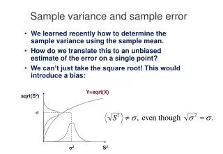
Y=sqrt(X). sqrt(S 2 ). . 2. S 2. Sample variance and sample error. We learned recently how to determine the sample variance using the sample mean. How do we translate this to an unbiased estimate of the error on a single point?

Sample variance and sample error
E N D
Presentation Transcript
Y=sqrt(X) sqrt(S2) 2 S2 Sample variance and sample error • We learned recently how to determine the sample variance using the sample mean. • How do we translate this to an unbiased estimate of the error on a single point? • We can’t just take the square root! This would introduce a bias:
Mean and variance of S2 • Like any other statistic, S2 has its own mean and variance. • Need to know these to compute bias in S:
Bias in sqrt(S2) • Define square root function g: • g(X) and its derivatives: • Hence compute bias:
Unbiased estimator for • Re-define bias-corrected estimator for :
Y P(Y|X) P(Y) X P(X) P(X|Y) Conditional probabilities • Consider 2 random variables X and Y with a joint p.d.f. P(X,Y) that looks like: • To get P(X) or P(Y), project P(X,Y) on to X or Y axis and normalise. • Can also determine P(X|Y) (“probability of X given Y”) which is a normalised slice through P(X,Y) at a fixed value of Y or vice versa. • At any point along each slice, can get P(X,Y) from:
Bayes’ Theorem and Bayesian inference • Bayes’ Theorem: • This leads to the method of Bayesian inference: • We can determine the evidence P(data|model) using goodness-of-fit statistics. • We can often determine P(model) using prior knowledge about the models. • This allows us to make inferences about the relative probabilities of different models, given the data.
X P(X|a) Uniform P(a) P(a)~1 / Log (a) P(a|X) P(a|X) Choice of prior • Suppose our model of a set of data X is controlled by a parameter . • Our knowledge about before X is measured is quantified by the prior p.d.f. P(). • Choice of P() is arbitrary subject to common sense! • After measuring X get posterior p.d.f. P(|X) = P(X|).P() • Different priors P() lead to different inferences P(|X)!
X P(X|a) Uniform P() P()~1 / Log () P( |X) P( |X) Examples • Suppose is the Doppler shift of a star. • Adopting a search range –200 < < 200 km/sec in uniform velocity increments implicitly assumes a uniform prior. • Alternatively: scaling an emission-line profile of known shape. • If you know ≥ 0, can force > 0 by constructing the pdf in uniform increments of Log so P() ~ 1/Log(). • Posterior distributions are skewed differently according to choice of prior.
Relative probabilities of models • Two models m1, m2 • Relative probabilities depend on • Ratio of prior probabilities • Relative ability to fit data • Note that P(data) cancels.
Maximum likelihood fits • Suppose we try to fit a spectral line + continuum using a set of data points Xi, i=1...N • Suppose our model is: • Parameters are C, A, 0, • i , i assumed known.
Likelihood of a model • Likelihood of a particular set of model parameters (i.e. probability of getting this set of data given model ), is: • If errors are gaussian, then:
350 300 250 200 -2 ln L 150 100 2N ln 50 0 0 10 20 Estimating Xi • Data points Xi with no errors: • To find A, minimise 22. • Can’t use 2 minimisation to estimate because : • Instead, minimise i