Watershed Management Runoff models
Watershed Management Runoff models. Hydrology and Water Resources, RG744 Institute of Space Technology November 13, 2013. Runoff models. Peak runoff models Provide only the estimates of peak discharge from the watershed Continuous runoff models


Watershed Management Runoff models
E N D
Presentation Transcript
Watershed ManagementRunoff models Hydrology and Water Resources, RG744 Institute of Space Technology November 13, 2013
Runoff models • Peak runoff models • Provide only the estimates of peak discharge from the watershed • Continuous runoff models • This class of runoff models provides storm hydrographs for a given rainfall hyetograph • Provide an estimate of runoff vs. time series
Peak runoff models • Rational Method • NRCS Method
Rational Method • To calculate peak runoff from small watersheds • Provides peak runoff rate from a catchment given: • the runoff coefficient C, • the time of concentration Tc, • the area of the catchment, and • the information to calculate the input or design storm or rainfall event
Rational Method: Assumptions • Catchment is small (less than 200 acres) • Catchment is concentrated • Rainfall intensity is uniform over the area of study • The runoff coefficient is catch-all coefficient that incorporates all losses of the catchment
Rational method: formula Qp = CIiA • Qp = Peak discharge (cfs) • C = runoff coefficient (function of soil type and drainage basin slope) • Ii = average rainfall intensity (in/hr) for a storm duration equal to the time of concentration, Tc • A = area (acre) • For runoff coefficient refer Bedient Table 6-5 page 381 • Obtain i from IDF curve with tr (duration) and T defined (assume tr = Tc)
Determining Tc • Take Tc = 5min when A (acres) < 4.6 S (slope %) • Or use Kinematic Wave Theory (iterative process) • L = length of overland flow plane (feet) • S = slope (ft/ft) • n = Manning roughness • Ii= Rainfall intensity (in/hr) • C = rational runoff coefficient
Rational Method: example 6-6 Bedient • Drainage design to be accomplished for a 4 acre asphalt parking lot in Tallahassee for a 5 yr return period. The dimensions are such that the overland flow length is 1000 ft down a 1% slope. What will be the peak runoff rate? • Refer Table 6-5, 4-2 & Figure 6-5 • Assume tr value, for that value read rainfall intensity from IDF curve. Calculate Tc using Kinematic wave theory. (iterate till tr = Tc)
Runoff coefficient for nonhomogeneous area • Weighted runoff coefficient based on area of each land use • Cw = ∑j=1n Cj Aj/ ∑j=1n Aj • Example McCuen page 381
NRCS Runoff Curve Number Methods • By the USA Soil Conservation Service (now called the Natural Resources Conservation Service), division of the USDA (USA Department of Agriculture) • To predict peak discharge due to a 24-hr storm event • Empirically derived relationships that use precipitation, land cover and physical characteristics of watershed to calculate runoff amount, peak discharges and hydrographs • More sophisticated approach than Rational Method
NRCS Curve number • Curve number is a coefficient that reduces the total precipitation to runoff potential, after “losses” • Evaporation • Absorption • Transpiration • Surface Storage • Higher the CN value - higher the runoff potential will be • It is essential to use the CN value that best mimics the Ground Cover Type and Hydrologic Condition
NRCS Rainfall-Runoff Equation • Following equation presents relationship between accumulated rainfall and accumulated runoff • Where: • Q = accumulated direct runoff (in. or mm) • P = accumulated rainfall (potential maximum runoff) (in. or mm) (24-Hour Rainfall Depth versus Frequency Values) • Ia = initial abstraction including surface storage, interception, evaporation and infiltration prior to any runoff occurring (in. or mm) • S = potential maximum soil moisture retention after runoff begins (in. or mm) • Note: for P ≤ Ia, Q = 0 Equation 1
potential maximum retention (S) • potential maximum retention (S) can be calculated using Equation 2 Where: • z=10 for English measurement units, or 254 for metric • CN = Runoff Curve Number • Generally, Ia may be estimated as Ia = 0.2 S Equation 3 • Substituting Ia value in Equation 1 Equation 2 Equation 4
Estimation of CN • Equation 4 (slide# 14) can be rearranged so the CN can be estimated if rainfall and runoff volume are known (Pitt, 1994) • The equation then becomes:
Curve Number CN • The principal physical watershed characteristics affecting the relationship between rainfall and runoff are • land use, • land treatment, • soil types, and • land slope. • NRCS method uses a combination of soil conditions and land uses (ground cover) to assign a runoff factor to an area (CN) • CN indicates the runoff potential of an area • Higher the CN, the higher the runoff potential • Soil properties also influence the relationship between runoff and rainfall since soils have differing rates of infiltration • Based on infiltration rates, the NRCS has divided soils into four hydrologic soil groups
Composite Curve Number • When a drainage area has more than one land use • When Composite CN is used • Analysis does not take into account the location of the specific land uses • drainage area is considered as a uniform land use represented by the composite curve number • can be calculated by using the weighted method
Hydrologic Soil groups • Hydrologic Group is a grouping of soils that have similar runoff potential under similar storm and cover conditions • Group A Soils: High infiltration (low runoff). Sand, loamy sand, or sandy loam. Infiltration rate > 0.3 inch/hr when wet. • Group B Soils: Moderate infiltration (moderate runoff). Silt loam or loam. Infiltration rate 0.15 to 0.3 inch/hr when wet. • Group C Soils: Low infiltration (moderate to high runoff). Sandy clay loam. Infiltration rate 0.05 to 0.15 inch/hr when wet. • Group D Soils: Very low infiltration (high runoff). Clay loam, silty clay loam, sandy clay, silty clay, or clay. Infiltration rate 0 to 0.05 inch/hr when wet. • Effects of Urbanization: Consider the effects of urbanization on the natural hydrologic soil group. If heavy equipment can be expected to compact the soil during construction or if grading will mix the surface and subsurface soils, you should make appropriate changes in the soil group selected. • Antecedent soil moisture conditions: AMC I, II and III
Antecedent soil moisture conditions-AMC • AMC is the preceding relative moisture of the pervious surfaces prior to the rainfall event • Low: when there has been little preceding rainfall • High: when there has been considerable preceding rainfall prior to the modeled rainfall event • ACM I (dry), ACM II (average) and ACM III (wet) • For modeling purposes, we consider watersheds to be AMC II, which is essentially an average moisture condition
CNs • A CN of 100 is to be used for permanent water surfaces such as lakes and ponds
Continuous Runoff Models • Time area method • Unit Hydrograph Techniques
Time Area Method • Develop to address non-uniform rainfall in large areas • Convert rainfall excess into hydrograph • Concept of time-area histogram is used • This method assumes that outflow hydrograph results from pure translation of direct runoff to the outlet at uniform velocity, ignoring any storage effects in the watershed • Watershed divided into subareas with distinct runoff translation times to the outlet • Subareas are delineated with isochrones of equal translation time (numbered upstream from the outlet)
Time Area Method • If a rainfall of uniform intensity is distributed over the watershed area, water first flows from are as immediately adjacent to the outlet • Percentage of the total area contributing increases progressively in time • Example : Surface runoff from area A1 will reach the outlet first, followed by contributions from A2, A3, …..and so on • Qn = RiA1+Ri-1A2+…….R1Aj • Qn= Hydraulic ordinate at time n (cfs) • Ri= excess rainfall ordinate at time i (ft/s) • Aj= time-area histogram ordinate at time j (ft2)
Example 2-2 from Bedient page 112 • Time area histogram method. The following is an example of the inflow for hour 5 using the 5 hour rainfall and 4 sub-basins. Assume constant rainfall intensity of 0.5in/hr
Unit Hydrograph (UHG) Theory • Unit Hydrograph of a watershed is defined as the direct runoff hydrograph resulting from a unit depth of rainfall excess (1 in or 1 cm) distributed uniformly over a drainage area at a constant rate for an effective duration • The effective rainfall is considered uniformly distributed within its duration and throughout the whole area of the basin • Uniquely represents storm-flow response (hydrograph shape) for a given watershed
Unit Hydrograph Theory: Assumptions • The effective rainfall is uniformly distributed within its duration • The effective rainfall is uniformly distributed throughout the whole area of the basin • The base period of the direct runoff hydrograph produced by effective rainfall of same duration (intensities may be different) are also same • The ordinates of the direct runoff hydrographs of a common base period are directly proportional to the total volume of direct runoff represented by the respective hydrographs • For a given drainage basin the hydrograph of runoff due to a given period of rainfall reflects the unchanging characteristics of the basin
Unit Hydrograph Theory: Assumptions 2 Basic Assumptions: • Time Invariance • Direct runoff response to a given effective rainfall in a catchment is time invariant, i.e. direct-runoff hydrograph (DRH) for a given excess rainfall in a catchment is always the same irrespective of when it occurs • Linear Response • Direct runoff response to the rainfall excess is assumed to be linear. Means if inputs x1(t), x2(t) cause outputs y1(t) and y2(t) respectively then an input x1(t) + x2(t) will cause an output y1(t) + y2(t). Also if x1(t) = r x2(t) then y1(t) = r y2(t).
Linear Response • UH is 1/2 the size but TB (time base) and TP (time to peak) are the same
Properties of unit hydrograph • Volume under unit hydrograph is equal to 1 unit rainfall excess (1 in or cm) • If duration of 2 rainfall excess events is equal without regard to their respective rainfall intensities, they must result in the same hydrograph time base • Results in a linear system whereby the direct runoff for storm of specified duration is directly proportional to the rainfall excess amount or volume • Rainfall distribution for all equal duration storms is identical in time and space
Development of UHG • Examine records of watershed for single peaked, isolated stream flow hydrographs resulting from short duration rainfall hyetograph of relatively uniform intensity • Determine depth of storm precipitation spread over the watershed equivalent to the volume of water divided by area • Volume is equal to area under hydrograph • Ordinates of UHG can be calculated by dividing the ordinates of the DRH by the storm depth • Check: recalculate area under UHG and divide it by watershed area. That should give unit storm depth.
Example: • Determine the UHG ordinates for the hydrograph shown in figure. The area of watershed is 16.2 square km
Drg ordinates from uhg with Variable Rainfall excess values (M pulses of excess rainfall • Discrete Convolution Equation is used to compute direct runoff hydrograph ordinates • Qn = direct runoff hydrograph ordinates, Pm= Rainfall excess, Un-m+1 = unit hydrograph ordinates, • n= direct runoff hydrograph time interval (1, 2, …N), m= precipitation time interval • M = pulses of excess of rainfall N = pulses of direct runoff N-M+1 = L, Number of UH ordinates • Reverse process is called ‘deconvolution’ to derive unit hydrograph given Pm and Qn