Deterministic Global Parameter Estimation for a Budding Yeast Model
270 likes | 295 Vues
T.D Panning*, L.T. Watson*, N.A. Allen*, C.A. Shaffer*, and J.J Tyson + Departments of Computer Science* and Biology + , Virginia Tech Blacksburg, VA 24061. Deterministic Global Parameter Estimation for a Budding Yeast Model. Outline. Application: Cell Cycle Modeling

Deterministic Global Parameter Estimation for a Budding Yeast Model
E N D
Presentation Transcript
T.D Panning*, L.T. Watson*, N.A. Allen*, C.A. Shaffer*, and J.J Tyson+ Departments of Computer Science* and Biology+, Virginia Tech Blacksburg, VA 24061 Deterministic Global Parameter Estimation for a Budding Yeast Model
Outline • Application: Cell Cycle Modeling • Optimization Techniques: • Dividing RECTangles (DIRECT) • Mesh Adaptive Direct Search (MADS) • Computational Results
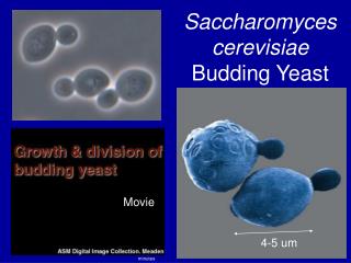
Application:Cell Cycle Modeling • How do cells convert genes into behavior? • Create proteins from genes • Protein interactions • Protein effects on the cell • Our study organism is the cell cycle of the budding yeast Saccharomyces cerevisiae.
cell division mitosis (M phase) G1 G2 DNA replication (S phase)
Modeling Techniques • We use ODEs that describe the rate at which each protein concentration changes • Protein A degrades protein B: … with initial condition [A](0) = A0. Parameter c determines the rate of degradation.
Tyson’s Budding Yeast Model • Tyson’s model contains over 30 ODEs, some nonlinear. • Events can cause concentrations to be reset. • About 140 rate constant parameters • Most are unavailable from experiment and must set by the modeler • “Parameter twiddling” • Far better is automated parameter estimation
Mutations • Wild type cell • Mutations • Typically caused by gene knockout • Consider a mutant with no B to degrade A. • Set c = 0 • We have about 130 mutations • each requires a separate simulation run
Phenotypes • Each mutant has some observed outcome (“experimental” data). Generally qualitative. • Cell lived • Cell died in G1 phase • Model should match the experimental data. • Model should not be overly sensitive to the rate constants. • Overly sensitive biological systems tend not to survive
Transforms • The output from ODE solvers are time course data • Need to convert this to match the qualitative experimental data • We call the function that does this conversion a “transform”
Rules of Viability • Modeled cell must execute a series of events, in order • [Clb2] + [Clb5] drops below Kez2. • [ORI] goes over 1 before two divisions of wild cell. • [SPN] increases above 1. • [Esp1] increases above 1. • [Clb2] drops below Kez. • Cell is inviable if [BUD] does not reach 0.8 before (e) • Squared relative differences of masses and G1 phase lengths in last two cycles is less than 0.5. • Cell is inviable if mass has higher ratio than 4 to wild cell.
Organizing the Observations Budding yeast phenotype for a given mutant is defined by a 6-tuple (v, g, m, a, t, c). • v is {viable, inviable} • Real g > 0 is steady state length of G1 phase • Real m > 0 is steady state mass at division • a (arrest stage) is {unlicensed, licensed, fired, aligned, separated} • Integer t > 0 is the arrest type • Integer c >= 0 is number of successful cycles Define 6-tuples O (observed) and P (predicted).
Objective Function • We require a scoring mechanism to compare O and P for each mutant.
Objective Function (cont) • The constants are tuned such that a rating of around 10 for a given mutant is a critical error (the model effectively fails for that mutant) • Note that this objective function is not continuous
Optimization Techniques • 143 parameters to optimize • DIviding RECTangles (DIRECT) • Global optimization • Mesh Adaptive Direct Search (MADS) • Local optimization
DIviding RECTangles (DIRECT) • Global optimization algorithm (Jones et al, 1993) • Does not require gradient, but the convergence criteria does require the objective function to be continuous • At each iteration, subdivide boxes considered to be “potentially optimal” into three along their longest dimensions • The algorithm can be tuned to favor “exploration” for good regions, or focus on known good regions
Mesh Adaptive Direct Search (MADS) • A class of algorithms • Alternate SEARCH and POLL steps. • All evaluated points are on a mesh, but the mesh can be adjusted each iteration. • Each SEARCH step selects some points on the mesh to evaluate. If an improved point is found, MADS may jump directly to resizing the mesh. (GPS) • If no better point is found in the SEARCH step, the POLL searches for a better point within a fixed distance (the frame) of the current best point. (Frame – Coope & Price) • Resize the mesh up or down depending on success in the last iteration.
Computational Results • All computation took place on Virginia Tech’s System X supercomputer • We used parallel implementations for DIRECT and MADS. • Experiment 1 • MADS started from the modeler’s best point • DIRECT used a box normalized around the modeler’s best point
Experiment 1 • MADS evaluated 135,000 points (813 iterations, 128 processors). Final objective function value was 299. • DIRECT evaluated 1.5M points (473 iterations, 1024 processors). Final objective value was 212.
Experiment 2 • Looking at the results of Experiment 1, DIRECT does not progress much after 200,000 points. • What if we start MADS from this point? • What about other points on the plateau? • Mixed results: • The MADS runs starting at the beginning and end of the plateau were worse than DIRECT’s best point. • The MADS run starting in the middle of the plateau was better than DIRECT’s best point. • MADS made effectively no progress when starting from DIRECT’s best point.
Contributions • Demonstrated that it is computationally feasible for search algorithms to improve on the modelers’ best point. • The best points found by DIRECT were more stable than the modelers’. • MADS can (sometimes!) improve on DIRECT when starting from DIRECT’s good points. The relationship is unclear. • Demonstrated the relationship in DIRECT’s tuning parameter of tradeoff between splitting large boxes and refining small boxes.