Download
1 / 47
480 likes | 602 Vues
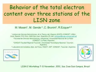
Behavior of the total electron content over three stations of the LISN zone. M. Mosert 1 , M. Gende 2 ,C. Brunini 2 , R.Ezquer 3,4

E N D
Behavior of the total electron content over three stations of the LISN zone M. Mosert1, M. Gende 2 ,C. Brunini2, R.Ezquer3,4 1 Instituto de Ciencias Astronómicas, de la Tierra y del Espacio (ICATE)-CONICET- UNSJ, Avda. España 1512 (Sur), 5400 San Juan, Argentina, [E-mail: mmosert@icate-conicet.gob.ar] 2Facultad de Ciencias Astronómicas y Geofísicas, Universidad Nacional de La Plata- CONICET, La Plata, Argentina 3CIASuR, Facultad Regional Tucumán, Universidad Tecnológica Nacional, Tucumán, Argentina. 4 Laboratorio de Ionósfera, Dpto. de Física, FACET, UNT- CONICET, Tucumán, Argentina LISN 2 Workshop 7-11 November, 2011, Sao Jose Dos Campos, Brazil
In this talk We analyze the behavior of total electron content using data from Jicamarca (-12.0°S; 283°E); Tucuman (-26.9°S; 294.6°E) and El Leoncito, San Juan (-31.5°S; 290.4°E). The database includes TEC measurements obtained from Digisonde observations (ITEC) and GPS signals (GPSTEC). The day to day variability is analyzed. Comparisons between observations and the IRI –2007 predictions are also done.
Data Used Station Lat. Long. Years Rz12 Jicamarca -12.0° S 283° E 2001-2008 HSA-LSA Tucuman -26.9°S 294.6°E 2008 LSA El Leoncito -31.5°S 290.4°E 2008 LSA Representative months: January (summer), April (fall), July (winter) and October (spring) Universal Time: 00 to 23
Data Used ITEC:(h= 1000 km) obtained from digisonde ionograms using the true height inversion program NHPC (Reinisch and Huang, 1983; Huang and Reinisch, 1996) GPSTEC:Vertical TEC derived from oblique GPS signals using La Plata Ionospheric Model, LPIM (Brunini et al, 2001) IRITEC:(h =1000 km) obtained from IRI-2007 version (3 Topside options: IRI-2001, IRI-2001 corrected and NeQuick).
Our analysis Behavior of GPSTEC over Jicamarca , Tucumán and El Leoncito, San Juan Behavior of ITEC over Jicamarca Analysis of topside electron density profiles
2. Behavior of ITEC over Jicamarca Seasonal Variations Solar Activity Variations Day to Day Variability Comparisons between observations and IRI predictions
ITEC – Median or Mean values? Jicamarca 2002 (Rz12= 102) Fig. 3 F
Jicamarca 2006 (Rz12=16) Fig. 4
Jicamarca ITEC Seasonal Variations 2006 (Rz12= 16) – 2002 (Rz12= 102) Fig. 8
Day to Day Variability Variability indexes Standard Deviations (SD) V%: Standard Deviations % = (SD/mean) * 100 Upper and lower quartiles Cup= upper quartile/median Cup >1 Clo= lower quartile/median Clo <1 Variability index: Cup-Clo
Jicamarca - ITEC – 2006 (LSA: Rz12= 16) Variability indexes Cup and Clo Fig. 11
Jicamarca - ITEC – 2002 (HSA: Rz12= 102) Variability indexes Cup and Clo Fig. 12
Jicamarca – ITEC – 2002 (HSA) / 2006(LSA) Variability index V% Fig. 13
Jicamarca 2002 – ITEC / IRITEC Fig. 15
Jicamarca 13/11/2001 (Rz12= 111) Fig. 16
Jicamarca 11/06/2002 (Rz12= 102) Fig. 17
Jicamarca 15/04/2004 (Rz12= 42) Fig. 18
Jicamarca 28/06/2006 (Rz12= 16) Fig. 19
Jicamarca 30/06/2006 (Rz12= 16) Fig. 20
A study of the behavior of the total electron content (TEC) has been done using measurements obtained at Jicamarca, Perú (12.0 S; 283.0 E) and at Tucumán (26.9 S; 294.6 E ) and El Leoncito, San Juan (31.5 S; 294.6 E ), Argentina. The database includes TEC data derived from ground-based ionosonde data (ITEC) and from GPS satellite signals (GPSTEC). The diurnal, seasonal, solar activity variations and the day to day variability have been analyzed. Comparisons with the predictions of the last version of the International Reference Ionosphere model (IRI-2007) are also done. The results show that the total electron content increases gradually from hours of minimum TEC (05-06 LT) in all the seasons reaching maximum values around midday. At sunset the TEC values begin to decrease reaching minimum values around sunrise. The TEC measurements generally show lower values in winter than in summer. The winter-summer differences are not so evident in the year of low solar activity. The largest daytime peak values are observed in the two equinoctial months.The IRI predictions generally overestimate the total electron content during nighttime and underestimate during daytime.Taking into account that the most contribution of TEC comes from the topside electron density profile, these results suggest that the discrepancies between IRI predictions and TEC measurements are due to the shape of the topside profile assumed by the model. In general NeQuick topside option follows better the ISR data. Summary
Final Comments • Takingintoaccounttheseresultsadditionalefforts are being done in order: • Toimprovethemodeling of theelectrondensityprofile. • (b) Toadvance in theformulation of a daytodayvariabilitymodel. • and somecommentsaboutthe new ionosoneinstalled at Tucuman.
Operativeionosphericstations Tucumán 2 (CIASUR- FRT and UTN) La Plata (GESA-UNLP) B. San Martin B. Belgrano (IAA)
Tucumán (-26.9º S , 294.6º E) is placed near the Southern crest of the equatorial anomaly. Since 1957 to 1987 ionospheric measurements were obtained with the analogue ionosonde of the Ionospheric Station of National University of Tucumán (UNT). In 2007, within the Italian-Argentine collaboration supported by the Istituto Italo Latino Americano (IILA), an Advanced Ionospheric Sounder (AIS) built at the Istituto Nazionale di Geofisica e Vulcanologia (INGV), Rome, was installed at the Upper Atmosphere and Radiopropagation Research Center (Centro de Investigación de Atmósfera Superior y Radiopropagación – CIASUR) of the Tucumán Regional Faculty of the National Technological University (UTN). That ionosonde is equipped with Autoscala, software able to perform an automatic scaling of the ionograms. Figure 1 shows AIS, the antenna and an ionogram obtained at CIASUR.
SF and Scintillations 1:45 UT Satélite 2 22:45 LT 1 1:30 2 2:30 UT
3:45 UT Satélite 23 0:45 LT
4:00 UT Satélite 13 1:00 hs LT
The data recorded by the AIS-INGV/Autoscala system installed at CIASUR showed ionograms with possible additional stratifications, different to E, F1 and F2 layers (Pezzopane et al 2007). Fig. 2 shows an example were a F1.5 additional stratification is observed. First results
Fig. 2. Ionograms recorded on 23 September 2007 from 14:05 to 14:45 UT by the AIS-INGV ionosonde installed at Tucumán, and autoscaled by Autoscala. The development and decay of a F1.5 additional stratification are highlighted using open circles. (From Pezzopane et al 2007)
Range spread-F (RSF) and occurrence of “satellite” traces prior to RSF onset were also studied with AIS measurements. (Cabrera et al., 2010). Fig. 3 shows a case where ST and RSF are observed. First results
Fig. 3. Sequence of ionograms recorded on 4 September 2007 showing (a) diffuse trace in the second order mode, (b) ST appearance adjacent to the low- frequency end of the first order mode, (c) RSF commencement, and (d) RSF fully developed. (From Cabrera et al, 2010)
Acknowledgments We gratefully acknowledge to FAPESP for the financial support and to INPE for hosting this event in particular to Eurico di Paula. The authors wish to thank to the staff of the JRO for the use of ISR data.