Topics in Labor Supply
351 likes | 678 Vues
Topics in Labor Supply. Chapter 3. Extensions of Static Model. Labor supply over the lifecycle Fertility Household production Retirement Policy: Decline in work attachment among older workers. Labor Supply over the Lifecycle.

Topics in Labor Supply
E N D
Presentation Transcript
Topics in Labor Supply Chapter 3
Extensions of Static Model • Labor supply over the lifecycle • Fertility • Household production • Retirement • Policy: Decline in work attachment among older workers
Labor Supply over the Lifecycle • Workers can “save” earnings when H* is high and enjoy more C and L later in life • Age-earnings profile • OC of leisure _____ when young and old • OC of leisure _____ during “prime” working years “Inverse U” • Note: Workers anticipate evolution of wages, so high wages during prime years do not increase lifetime income
Labor Supply over the Lifecycle • Given age-earnings profile, younger and older workers enjoy leisure more than prime age workers • H* and w • In the lifecycle model, an increase in w is expected (evolutionary ∆wOC of leisure), but does not increase lifetime income (lifetime opportunity set)
Labor Supply over the Lifecycle • Recall: In the lifecycle model, an increase in w is expected and only induces a substitution effect for a particular worker • Comparing the level of two wage profiles generates an income effect • Jeff’s hours profile = Jeff if substitution effect dominates • Jeff’s hours profile = Jeff if income effect dominates
LFPR over the Lifecycle • Reservation wage: in years when w > , people will work • less likely for younger and older workers, so it is as young and old ages that LFPR tends to be lower (than at prime-age years) • changes over the lifecycle (# children, etc), so LFP varies over the lifecycle
Empirical Evidence • Should show ↑ LFPR and ↑ H* when wages are high • Intertemporal Substitution hypothesis: • LFP • Males: participation peaks between ages 20 and 50 • Females: participation peaks during early 40s • Substantial decline after age 50 – retirement, health, disability insurance programs, etc. • Hours worked • Males: increase to age 30, decline after age 50 (2100 annual during prime years) • Females: peak during 40s (many PT before)
Fertility • Evidence: as per capital income rose, fertility rates have declined • Model: • N = number of children (will depend upon income and prices) • X = quantity of goods and services • pN = price of another child (~100K including foregone earnings) • pX = price of consumption goods • I = income • At tangency,
Comparative Statics • Suppose I↑, ceteris paribus • If children are a normal good, N*
Comparative Statics • Suppose pN↑, ceteris paribus • Income Effect: _ to _ • Substitution Effect: _ to _ • Income and substitution effects ____________
Empirical Evidence • Theory suggests the demand for children will __crease with wages [corr(income , N*) _ 0] or with a __crease in the cost of raising children [corr(pN , N*) _ 0] • Strong negative correlation between mother’s wage and the number of children (10% in wages decreases N* by 3%) • Weak negative correlation between N* and income (10% increase in wages decreases N* by 0.4%) • Why?:
Household Production • Model • Leisure = childrearing, cooking, cleaning, etc. • Household production yields commodities consumed in the household such as meals household production is an input to these commodities • Evidence • Labor market activity – Married men: 40 hours; Single men: 33 hours • Women allocate fewer hours than men to the labor market. • Married women allocate fewer hours than single women to the labor market. • Household production – Married women: 35 hours; Married men: 14 hours
Household Production, cont. • Goal: Determine how households allocate time to the labor market and to household production • Determined by comparative advantage: • Spouse with lower wage rate or greater household productivity specializes in __________ • Production Possibilities frontier
Household Production, cont. • OC of $1 of HH goods = slope = = $ of market good production • OC of $1 of HH goods = slope = = $ of market good production • Tim has a comparative advantage in __________________, and Jane has a comparative advantage in _____________________
Household Production, cont. • Joint PPF • Case 1: Jane and Tim both work in the labor market • Case 2: Jane and Tim both work at home • Case 3: Specialize
Household Production Decision • Who does what? • Depends where joint PPF and indifference curves are tangent • A: flat indifference curve (households enjoy market goods, so must work outside home) • B: households enjoy both goods • C: steep indifference curve (households enjoy goods produced at home)
Comparative Statics • Suppose Jane’s wage increases • Her contribution to the PPF becomes __________. • Tim’s productivity at home remains the same ($360, and slope does not change) • Jane will work ______ in the market and may eventually only work in the labor market
Comparative Statics • Suppose Tim’s home productivity increases • His contribution to the PPF ________________. • Jane continues to earn a maximum of $210 in the labor market. • Tim will spend _______ time on household production and may eventually only work at home.
HH Production Empirical Evidence • Gender differentials • Wage gap is shrinking • Improvements in household technology decrease the household productivity differential • 10% increase in wages (OC of HH production) HH hours decrease by 2% • When wage↑, HH production is less valuable and OC of leisure↑ LFP ↑ • Technological advances reduce HH productivity relative to labor market productivity, so HH hours ↓ (H*↑), primarily for women
Retirement • Model • Assume H = 0 after retirement (no PT work) • After retirement, individuals spend previous savings and employer-provided and/or government-provided pension benefits • More can be consumed by those who work longer since incomes usually exceed pensions • Tradeoff between leisure (longer retirement) and consumption budget constraint downward sloping • Determinants of retirement age: • Wage • Pension benefits
Retirement Decision • Assume someone who lives to age 80 decides to retire sometime between age 60 and age 80 • Vt =
Comparative Statics • Suppose w↑, benefits constant • If worker retires when wage increase goes into effect, the increase • If retirement is delayed until after wage increase, • Here, _____________ effect dominates
Comparative Statics • Suppose benefits↑, wage constant • If years of retirement = 0, • Income effect: • Substitution effect: • Years of retirement __crease
Retirement Empirical Evidence • LFPR of older men (ages 55-64) decreased between 13 and 35 percentage points between 1960 and 1996 • Theory: • 10% increase in wages reduces prob(retire before 65) by 6 percentage points ______________ effect dominates • Higher benefits _________ retirement • 10% increase in benefits reduces retirement age by 1 month
Shortcomings of Model • Model does not • In US, changed from age 65 to 70 in 1978 • Abolished in 1986 • Model does not • SS: 9% per year increase if individual retires between 62 and 65, additional 4% per year after age 65 • 2/3 of men retire between 62 and 65
Policy Application: Labor Supply Response to Child Care Subsidies • Examples: school lunches, day care subsidies, tax credits • 40% of American families utilize day care totaling, on average, 7% of income • Example 1: Reduce hourly cost of day care (assume no fixed cost component) • H* will
Policy Application: Labor Supply Response to Child Care Subsidies • Example 2: Reduce fixed costs (assume no variable cost) • Equivalent to an increase in non-labor income (V) • Non-workers
Policy Application: Labor Supply Response to Child Care Subsidies • Example 2, cont.: Reduce fixed costs (assume no variable cost) • Equivalent to an increase in non-labor income (V) • Workers • Summary: Subsidies should __crease LFPR and __________ _____________effect on H* • Empirical evidence supports LFP prediction, especially among low income workers
Policy Application: Decline in Work Attachment Among Older Workers • Why has LFPR among older workers (men) ↓? • ________: Life expectancy at age 50 of white men rose from 22 to 26.7 years • ___________________________: 26% covered in 1950, 66% in 1990 • Prob(men aged 58-63 with private penions work) ↓ by 18 percentage points • ______________________: rose in 1970s and remained constant (when real wages ↓) in 1980s, but at most 15% of LFP ↓ attributable to SS • ______________________: disabled worker receives SS benefits as if he/she retired at age 65, regardless of when disability occurred • Recipients (age 55-64) of DI increased from 3.5% to 10.5% between 1960 and 1985 • Mixed evidence regarding effect of DI in LFPR
Policy Application: Decline in Work Attachment Among Older Workers • Social Security Earnings Test • Provision of SS system which discourages recipients (aged 65-69) from working • Workers can earn up to $17K without affecting benefits • Earnings beyond $17K taxed $1 for every $3 earned (33% tax rate) • Workers over age 70 unaffected
Policy Application: Decline in Work Attachment Among Older Workers • How does the SS Earnings Test affect H*? • Worker A: • Worker B: • Worker C:
Policy Application: Decline in Work Attachment Among Older Workers • Empirical Evidence on the effect of the elimination of the SS Earnings Test on H* • Only individuals working a moderate number of hours would increase the number of hours worked (because of the substitution effect) • 20% of retirees work, and 60% of those workers are affected by the SS earnings test • Estimate: removing the Earnings Test would increase H* by approximately 1 hour per week (from 3.2 to 4.4 hours)
