Download
1 / 36
370 likes | 636 Vues
Labor Supply and Demand. In this section we study the general overall condition in labor markets. Labor supply. The supply curve for labor is an upward sloping curve from right to left. Why is the supply curve upward sloping?

E N D
Labor Supply and Demand In this section we study the general overall condition in labor markets.
Labor supply The supply curve for labor is an upward sloping curve from right to left. Why is the supply curve upward sloping? The logic is that people are willing to supply a greater amount of labor the higher the wage? Why do they need a higher wage to supply more labor? Leisure is a good thing, but it does not pay very much - like nothing dude and dudettes :). So, if your option is to work at a low wage or have leisure, you might take leisure. But if the wage is higher, you may be willing to give up the leisure to capture the higher wage. By the way, I am not saying you are a lazy bum if you do not work at low wages. You may go to school, retire, work for the peace corps or volunteer at schools, parks, churches or even visit the lonely. These are all great things! Our theory simply says at low wages we are not willing to give up fun stuff to work. But at a higher wage we might give up this stuff for the world of work.
Labor Supply To be a little more formal than the previous slide, recognize in a broad sense that the day is made up of hours of work and hours of leisure. In the area of econ we usually focus on the leisure and note if leisure time changes so does hours of work. As the wage rises 1) The substitution effect of a wage increase means that hours of leisure now become more expensive in the sense of the opportunity cost (what is given up) and folks substitute away from things that become more expensive. This means take less leisure, and more work.
Labor Supply 2) Income effect of a wage change means that if leisure is a normal good (meaning more income will have us take more of the good – and we do assume leisure is a normal good) a higher wage will mean more income and more leisure, and less work. Summary so far – a higher wage means more work due to substitution effect, and less work due to income effect. The income and substitution effects work in opposite directions. But, at low wages wage increase initially have the substitution effect as the stronger of the 2 and thus the supply is upward sloping. As the wage continues to rise at some point the income effect becomes stronger and the labor supply curve “bends” backwards.
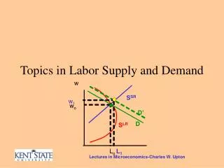
Labor Supply In the top graph we have the labor supply that has the sub effect stronger than the income effect all the time. In the bottom graph the income effect does overcome the sub. effect. In the whole market we horizontally add up all the individual supplies. In that setting, even if some folks have a backward bending supply, when adding across all people the market supply curve is often upward sloping. W Labor amount L W L
Derived demand • Resources or inputs are used to make products. The desire to use the input is derived from the desire to make the output. The input isn’t desired in and of itself. • How much of an input a firm wants is influenced by profits, but more specifically by • the productivity of the input • the selling price of the output made with the input • the price of the input • other factors not mentioned here.
Labor • Initially, we will focus on the demand for labor. • We will look at the case of labor demand where the firm sells output in a competitive environment, meaning it is an output price taker. • The firm buys the input in a competitive setting. The firm buys such a small amount of labor relative to the market that the firm is a input price (the wage) taker.
Overview Firms or businesses are profit maximizing entities (or so assumed in economics). As such, the only reason labor is demanded is because labor helps produce the goods and services the firm wants to sell. Labor demand is a derived demand – derived from the firms desire to sell output. In this section we study some economic concepts that influence how much labor the firm desires.
The production function We will assume that firms employ both labor and capital in the production process, one type of output is made, the quality of workers is basically the same, and our emphasis is on the number of workers demanded. In a shorthand notation we say q = f(L, K) Where q = the amount of output, L = the amount of labor used, K = the amount of capital used, and f means output is a function of, or depends on, the amount of capital and labor used.
Marginal Product The marginal product of labor – MP– is defined as the change in output resulting from hiring an additional worker, holding constant the quantities of other inputs used. We usually calculate a number to tell us about MP for each unit of labor. Take the change in output and divide by the change in labor, taking labor one unit at a time.
Cookie factory Imagine this room is a cookie factory - like at a shopping mall. The fixed input, or capital, is the production facility and it includes a certain number ( say two of each, for now) of refrigerators, bowls, mixers, ovens, tables and other stuff. The variable input will be labor. We will observe output levels at various levels of labor used. If the amount of capital were to change, we would likely have a whole new set of numbers.
Example continued This is just an example where we have added labor to a fixed amount of capital. Total output in this example will be measured in dozens of cookies per hour.
MP or marginal product • MP is the additional output from adding the additional worker. Note we go from line to line. • As more of the variable input is used with a fixed input, the marginal product first increases, reaches a maximum, then diminishes and even becomes negative.
MP - continued • MP is a max. at 2 units of labor and begins to diminish with the 3rd unit of labor. • As more labor is added there is less and less tools - capital - to use, so additional workers can not add as much output as previous workers.
AP or average product • At an output level AP = (total output)/(amount of labor used).
Law of diminishing returns You have probably noticed that the marginal product column first has a rising marginal product (as you go down the column and use more labor), then the marginal product reaches its peak, and then the marginal product declines – you should always use the word diminishes! What is the reason for this phenomenon? Economists believe, because of studies of the production process, when firms have a fixed amount of capital the first units of labor can specialize tasks and actually produce increasing returns, but at some point as more labor is added to the fixed amount of capital, there will not be as much capital for the additional workers to use and thus their contribution to output will diminish relative to the earlier workers.
Cookie factory again Have you ever made cookies without a mixer? If you have and then made some with a mixer you know how much nicer it is to use a mixer. Per time period you could make more cookies with a mixer than without one. Now, the more workers the more likely it is there are no mixers to use and thus additions to output diminish. By the way, here I am just talking about production possibilities at this one firm. The firm will end up doing only one of the possible amounts in a period of time.
Perfectly Competitive Firms For now we will assume that firms are too small to have the ability to make what price they would like to sell their output for or what price they would like to pay for labor or capital. This is the assumption of perfect competition in both the input market and the output market. The point here is some firms simply have to follow what is going on in the market, or they will not be able to survive. Let’s assume the output can be sold for $2 per unit. Marginal revenue in this setting is equal to price.
Marginal Revenue Product The marginal revenue of output (here = to price) times the marginal product is called the marginal revenue product(MRP). If you recall the property of diminishing returns you can see that the MRP follows the same basic pattern. Let’s look at that on the next screen.
Numerical example Remember we had assumed output price =$2
Marginal Revenue product dollars The MRP is basically telling us about revenue changes as we add workers, and hence output. Notice MR diminishes just like MP. MRP Number of workers
The cost of more labor Since the firm is a wage taker, ever time it uses another worker its cost goes up by the wage. In a graph similar to previous screen we have: The wage is telling us about how cost changes as we take on more workers. dollars wage Number of workers
Employment decision by the firm in the short run A firm that wants to maximize profit should always hire another worker if the revenue generated by that worker is greater than the cost of that worker and it should never hirer another worker if the revenue of that worker is less than the cost of that worker. What should it do in the case of a tie? We say hire that worker.
Employment decision by the firm in the short run dollars W1 W2 L1 L2 Number of workers
Employment decision by the firm in the short run On the previous slide I showed two wages. Remember the firm is a wage taker and therefore can not influence the wage. I just show two possible such wages. Once we have a wage we can see the firm would hire the amount of labor indicated on the value of the marginal product curve at that wage. The demand for labor by a firm is the downward sloping segment of the MRP curve.
The main points we want to get out of this section are understanding how much labor should the profit maximizing firm hire and what wage should it pay? We have just seen the demand for labor in the context of a firm that sells its output in a competitive market. If the output price should rise the value of the marginal product rises and thus the demand for labor shifts to the right. Similarly, if firms have technological change and workers become more productive the value of the marginal product rises and the demand shifts right. Now let’s think a little about the supply and demand together.
Wage determination On the next slide you see that the equilibrium wage and labor traded in the market is determined at the intersection of the supply and demand curves. Why is a higher price not an equilibrium? There would be an excess supply of labor and this would drive the wage down. Since this higher wage would change, we can not say it is an equilibrium wage. The next screen shows the market outcome and the decision of as a firm in the market. Note the market demand for labor is just the adding up of the demand from many firms.
Single labor market $ In the market we get wage W* and amount of labor traded L*. S W* D L L*
Equilibrium W* is the equilibrium wage because at this wage both suppliers and demanders obtain the desired amount. At wages higher than W* an equilibrium would not exist because at those wages the quantity supplied is much higher than the quantity demanded – an excess supply. All those willing to supply do not get to trade because there are too few buyers. Since this excess supply will encourage suppliers to change by lowering the wage at which many will work, the initial high wage (relative to the equilibrium) will not last and will change to the equilibrium wage.
More equilibrium At wages lower than W* an equilibrium would not exist because at those wages the quantity supplied is much lower than the quantity demanded – an excess demand. All those demanding do not get to trade because there are too few sellers. Since this excess demand will encourage demanders to change by raising the wage which they will pay for work, the initial low wage (relative to the equilibrium) will not last and will change to the equilibrium wage.
Changes in equilibrium The labor market model is similar to the basic model of supply and demand. Look at where the curves cross. Now, if demand rises the wage will rise and the amount of labor traded will rise. Before we said if the price of output rises or if the firm gets better technology the demand for labor will rise. Has the demand for pro sports gone up since 1970? I would say so. This probably is part of the reason for the increase in wages over time. If the supply rises the wage will fall and the amount traded will rise. How could the supply rise? Say many people from others countries move here – immigration. Then with more people living here the more likely it is that more will supply labor. So, the supply of labor curve shifts right the more people there are that want to work. We see here this pushes the wage down. Probably not a big factor in pro sports labor markets at this time.
Application: Productivity and Wages Remember the demand for labor is really the MRP curve of firms. Now say firms adopt better technologies and thus increase the MP of labor. The firms would thus have a higher MRP which would mean the demand for labor would rise. With a given supply of labor this would mean wages and employment would rise! So check this out, as firms use better technologies the wages of workers and the number of workers working rises. Who gives the workers the tools that have better technology? Firms do and thus when firms adopt better technologies they can pay workers more. Does it happen overnight? NO, they go home and sleep first and then later it kicks in!
Monopoly in the output market You may recall in a competitive market that firms are price takers. This meant that price is = marginal revenue. Then MRP = MR times MP = price times MP. In a monopoly market for output we know that MR < P. This means MRP = MR times MP < P times MP. The implication here is that if the market for output is monopoly the demand for labor is not as large as we had before and thus price and labor traded are lower amount. The other conclusions we made still hold though.
In the output market a monopoly wants to sell less than in competition and thus there is less labor traded and at a lower wage. W S Demand when output market is competitive Demand when output market is monopoly Quantity of labor