Labor Demand
Labor Demand. Chapter 4. Labor Demand Questions. Which workers should a firm hire? How many workers should a firm hire? How much capital? How will firms respond to employment subsidies? How should firms respond to policy changes such as minimum wages, affirmative action, etc?.


Labor Demand
E N D
Presentation Transcript
Labor Demand Chapter 4
Labor Demand Questions • Which workers should a firm hire? • How many workers should a firm hire? How much capital? • How will firms respond to employment subsidies? • How should firms respond to policy changes such as minimum wages, affirmative action, etc?
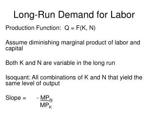
Production Function • Describes the technology used to produce goods and services • q = f(E,K) where • q = output • E = number of employee hours hired = number of workers x average hours per worker • K = capital – land, machines, other physical inputs • Assume homogenous workers (ignore education, etc) • Output is a function of the number of employee hours hired by the firm and the quantity of capital employed
Production Function, cont. • Recall: q = f(E,K) • Marginal Product: • MPE = • MPK = • MP = slope of total product curve • Interpretation:
Production Function Characteristics • TP increases rapidly, then at a decreasing rate • When TP increases at an increasing rate, MP • When TP increases at a decreasing rate, MP • When TP decreases, MP • Law of Diminishing Marginal Returns: • MP, AP relationship • AP increases when MP AP • AP decreases when MP AP • MP = AP at
Short Run Employment Decision • Firms goal: where • w = cost of hiring an additional worker • r = price of capital • p = output price • Short run: • E*: Choose E* such that • VMPE=P·MPE taken as given for PC firms
SR Employment Decision Example • Let w = $32, P=$3 • If E = 2, VMP = $33, but w = $32, so 3rd worker • If E = 3, VMP = $24, but w = $32, so 4th worker • w = $32 falls between VMP(E=1)=30 and VMP(E=2)=36, but • If law of diminishing MP did not hold, E* would have no bounds, so diminishing MP ensures firm can- not influence market
SR Employment Decision, cont. • Recall: • APE increases when MPE APE • APE decreases when MPE APE • MPE = APE at • VAPE = P∙APE is a “blown-up” version of APE, so VMPE = VAPE at • E* only valid if • If VMP(E*) = w > VAP(E*),
Individual Firm Demand Curve • Demand curve: Allow price (wage) to vary and determine how many employees the firm demands • If w = $15, E* = • If w = $21, E* = • If w = $24, E* = • SR demand curve for labor is:
Individual Firm Demand Curve, cont. • VMP curve drawn for a particular price, so when output price changes, VMP (labor demand) curve shifts • Positive relationship between P and the short-run demand for labor • Capital costs (r) constant, and when P↑, revenue ↑ • Firms only increase E* when revenue from new worker exceeds cost of worker (VMP > w)
Labor Market Demand Curve • Recall: Market labor supply curve derived by • Market Demand Curve • Roughly • Caveat:
Labor Market Demand Curve, cont. • Because of the caveat, the true labor market demand curve is ______ than the horizontal sum of individual demand curves
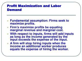
Profit Maximization Approach • Recall: Profit maximizing firms choose q* such that MR = MC, where • For a fixed K (short run condition), • For a PC firm, P = MR, so operating at MR = MC implies:
Objections to MP Theory • Note: • MP Theory: Choose E* such that w = VMPE • E* implies q* based on the production function • Employers do not really calculate VMPE and find where w = VMPE • Adding employees to the production process while holding K constant will not increase marginal productivity
Elasticity of SR Labor Demand • How responsive is labor demand to changes in wages? • __________ (by definition): When wages increase, firms demand ______ workers • Interpretation: • Elastic (_____ responsive) when |δSR| 1 • Inelastic (_____ responsive) when |δSR| 1
Long Run Employment Decision • Long run: • The firm can choose E* and K* • Isoquants: • Note: “iso” = equal, “quant” derived from quantity, so isoquant = “equal quantity”
Characteristics of Isoquants • Do not intersect • Downward-sloping • Higher isoquants represent _______ levels of output • Convex to the origin • When E is large, a _____ ∆K could replace many workers and maintain the same q • When E is small, a _____ ∆K would be required to maintain the same q
Characteristics of Isoquants, cont. • Slope: Move from point X to Y • Gain: • Loss: • To remain on the same isoquant, MPE∙∆E + MPK∙∆K = 0 • Slope = Marginal Rate of Technical Substitution (MRTS) • Interpretation: • Convexity implies diminishing MRTS
Isocosts (Constraint) • Isocosts: • Isocosts further away from the origin imply _____ costs • Cost = wE + rK
Profit Max/Cost Min • Profit max Cost min • Choose q* and produce at the lowest cost (isocost closest to origin) combination of K, E • Isocost-Isoquant tangency:
Profit Max/Cost Min, cont. • To profit max, firms choose q* such that MR=MC, then choose K* and E* to minimize costs • Recall: MR = MC implied w = P∙MPE; analogously, it also implies r = P∙MPK • Therefore, profit max implies cost min
Profit Max/Cost Min, cont. • So far, profit maximization implies cost minimization • Does cost minimization imply profit maximization? • Profit maximization Cost minimization, but • Cost minimization Profit maximization
Long Run Demand Curve for Labor • Recall: Demand curve is derived by allowing price (wage) to vary and determine how many employees the firm demands • Suppose initially, q*=q0 with C=C0 and w=w0 • Cost effect of w↓ • If w↓, firm may buy more labor and incur C=C0, • If C↑ to C1, holding constant r, the entire budget line
Long Run Demand Curve for Labor • Cost effect of w↓, cont. • With new cost (C1), new intercept = • Production effect of w↓ • When w↓, MC of production likely ________ (additional cost of producing one more unit ) • With _MC, MR _ MC at q0, so firm responds by _q • When w↓, E*_, K*_
Scale and Substitution Effects • So far, we’ve seen that when wages decrease, production costs (MC) __crease, so firms have an incentive to __crease production and hire _____ workers (E* ) • Substitution Effect • Capital is now a relatively ______________ input, so firms SUBSTITUTE away from ________ and toward a more _______-intensive production process (K* and E* ) • Scale Effect (eliminates the change in relative prices) • When firms produce more output (because of decreased MC of production), they may hire _____ employees and _____ capital simply because the SCALE of production changes (K* and E* )
Decomposing the Scale and Substitution Effects • To isolate the scale effect, draw a hypothetical isocost with same slope as original isocost and tangent to new isoquant • Scale Effect: __ to __ • Substitution Effect: __ to __ • As drawn, ___________ effect dominates, and K* • Note: Scale and substitution effects both suggest E*_, but the dominant effect determines how K* changes
Long Run Demand Curve for Labor • Recall: Both scale and substitution effects suggest E*_ when w↓ • Scale effect: When q↑, firm demands more K and more E • Substitution effect: Firms demand more of the relatively less expensive input when w↓ • Therefore, the LR demand curve for labor is _________ sloping (E*_ when w↓)
Elasticity of Labor Demand • δLR _ 0 because of the ______ relationship between w and E • δLR vs δSR: δLR _ δSR because firms can be more responsive to wage changes with fewer constraints (K not fixed in the long run) • Therfore, the LR demand curve for labor is ______ than the SR demand curve curve for labor
Elasticity of Labor Demand • Short-run elasticity of labor demand: • -0.5 < δSR < -0.4 • Long-run elasticity of labor demand: • δLR ≈ -1 • 1/3 due to the substitution effect, 2/3 due to the scale effect
Elasticity of Substitution • Perfect Substitutes • Here, 2K = 1E • Recall: Convexity of a “normal” isoquant implied • Here, inputs can be substituted at a ___________ rate • _________ substitution effect • One of the two extremes will be chosen (K = 100 OR E = 50, depending upon w and r)
Elasticity of Substitution, cont. • Perfect Complements • If E = 5, K = 5, can produce just as much output as E = 5 and K = 25 • To increase output, must add • Always use ____________ for q0, regardless of w and r • _____ substitution effect (___ substitutability) between K and E
Elasticity of Substitution, cont. • Elasticity of Substitution= • Measure of • When labor becomes relatively more expensive (w/r)↑, relatively ______ capital will be used (K/E) • Large elasticity of substitution means firms are _________ responsive to changes in relative input prices • More curved isoquants have _______ elasticities of substitution
Policy Application: Affirmative Action • Affirmative action encourages firms to alter the race, ethnicity, or gender of workforce by hiring relatively more of the workers typically under-represented in past hiring • Assume: • Two types of inputs – black and white workers • Black and white workers may have different education levels, skills, etc. • wB = black wage, wW = white wage
Policy Application, cont. • Case 1 • Note: Intercepts suggest wW _ wB • Point _ would be profit-maximizing (cost-minimizing) for a “color blind”, non-discriminating firm • A discriminating firm might choose point _ to have fewer black employees • A fine-tuned AA program could
Policy Application, cont. • Case 2 • Note: Again, intercepts suggest wW > wB • Firm may be non-discriminating and still hire relatively more whites (point _), perhaps because of productivity differences, etc. • An AA program may force the firm to hire relatively more blacks (point _), which is no longer profit-maximizing • Therefore, AA programs may improve profitability if the firm is ________________, but will reduce profits if firms are _____ __________________
Marshallian Rules of Derived Demand • Derived Demand: • What happens in the market for the good itself directly influences demand for labor (for instance, when P changes, VMPE (DE) shifts) • Marshallian rules describe factors which are likely to generate an elastic demand for labor
Marshallian Rules of Derived Demand • Rule 1: Greater elasticity of substitution between labor and capital (less curved isoquants) • Rule 2: Greater elasticity of demand for output • When wages ↑, the MC of production ↑, so supply ↓ and output P↑
Marshallian Rules of Derived Demand • Rule 3: Greater labor’s share of total costs of production • When labor is a large share of production costs, a wage change has a substantial impact on MC, on market supply (of output), and ultimately, on P
Marshallian Rules of Derived Demand • Rule 4: Greater supply elasticity of other inputs to production • When w↑, the firm will want to • If the price of that input increases dramatically when more is demanded, the incentive to replace labor with other inputs is ___________ • If the supply of the other input is ________ (relatively _____ supply curve), the increase in demand will result in only a moderate price increase, so firms will be more likely to make substantial changes in the relative share of inputs in the production process
Factor Demand with many inputs • So far, q =f(E,K) • Can add to the production function different types of workers, machines, etc. • q = f(x1,x2,…,xi,…xm) where • xi = quantity of input i • xi* determined by: wi=P∙MPi where • wi = cost per unit of input i (wage, rental rate, etc) • Results in the 2-input case hold in this more general set-up • Empirically, labor demand for unskilled workers is more elastic than the demand for skilled workers Labor market much more unstable for unskilled workers
Cross-Price Elasticity of Demand • How does the demand for input i (xi) respond to a change in the price of input j (wj)? • Cross-price elasticity of input demand • If inputs are substitutes (ηX-P _ 0), demand curve for input i shifts _____ in response to an increase in the price of good j) ____________ effect dominates • If inputs are complements (ηX-P _ 0), demand curve for input i shifts _____ in response to an increase in the price of good j) ___________ effect dominates
Empirical Evidence • Skilled and unskilled labor • Empirically, skilled and unskilled labor are _________ (ηX-P _ 0) • Unskilled labor and capital • Empirically, unskilled labor and capital are ________ (ηX-P _ 0) • Cross-price elasticity of input demand ≈ 0.5 • Skilled labor and capital • Empirically, skilled labor and capital are __________ (ηX-P _ 0) • Cross-price elasticity of input demand ≈ -0.5
Labor Market Equilibrium • Intersection of supply, demand defines (E*,w*) • If w > w*, QS _ QD competition drives w_ to w* • If w < w*, QS _ QD competition for workers drives w_ to w*
Application: Minimum Wages • Fair Labor Standards Act (FLSA) • Established in 1938 • Created a minimum wage, established overtime laws, child labor laws, etc. • Minimum wage: price ______ on wages (min w _ w*) • Higher wage has two effects • Unemployed =
Application: Minimum Wages, cont. • Recall: • With minimum wage, • Depends upon minimum wage, elasticities of S, D • UR higher when S, D more ________ (______ curves) suggests firms and/or workers are responsive to wage changes
Application: Minimum Wages, cont. • Empirical Evidence • Approximately 40% of workers who qualify for minimum wage are not paid it • Firms that are caught can delay paying a portion of payroll for two years (like an interest-free loan) and typically do not pay fines • Not all workers work in sectors covered by the minimum wage law (~10% in 1990)
Application: Minimum Wage, cont. • Workers in covered sector displaced by the minimum wage may move to the uncovered sector. • The equilibrium wage in the uncovered sector would __crease. • Note that the wage in the covered sector would also __crease due to ________ workers supplying their services to that market (not shown).
Application: Minimum Wage, cont. • Workers in uncovered sector may leave their current jobs to try to find new work in the covered sector to take advantage of minimum wage. • The equilibrium wage in the uncovered sector would __crease. • Note that the wage in the covered sector would also __crease due to an _________ in the number of workers supplying their services to that market (not shown).