Labor demand
Labor demand. Firm’s Demand in SR. Only labor input is variable while capital amount is fixed. Marginal revenue product (MRP) Additional revenue earned if employ one more unit of input

Labor demand
E N D
Presentation Transcript
Firm’s Demand in SR • Only labor input is variable while capital amount is fixed. • Marginal revenue product (MRP) • Additional revenue earned if employ one more unit of input • When factor price is fixed, MRP is obtained by marginal product of labor times marginal revenue of the output. (you need to be careful on this)
Firm’s Demand in SR Wage rate and MRP • Marginal product of labor is defined as the contribution to output by adding an additional unit of labor. • So the amount of labor needed to produce one more unit of output is: • And the cost of this amount is (this, by definition, refers to marginal cost of x):
Firm’s Demand in SR Wage rate and MRP • Now we know that when the firm maximizes profit, they set marginal revenue equal to the marginal cost: • So:
Firm’s Demand in SR Two major points drawn from the algebra: • It confirms that a profit-maximizing firm operates where the wage rate of labor is equal to its marginal product of labor. • The firm’s demand curve for labor coincides with the MRPL curve.
Some comparative statics • Wage goes up. • Output price goes up. • An increase in plant size
Some comparative statics • Wage goes up. • Output price goes up. • An increase in plant size
Some comparative statics • Wage goes up. • Output price goes up. • An increase in plant size
Recap Production and Costs in the Long Run • Firm can adjust employment of capital and labor • Achieve the least cost method of producing a given quantity of output
Isoquants • Geometry of LR production • Requires labeling vertical axis with K, stands for capital • Requires labeling horizontal axis with L, which stands for labor • Requires fixed period of time • Least costly method • Avoid technologically inefficient points which are outside the boundary • General observations about isoquants • Slope downward • Fill the labor-capital plane • Never cross • Convex to origin
Marginal Rate of Technical Substitution • Absolute value of slope of isoquant • MPL divided by MPK • Amount of capital necessary to replace one unit of labor while maintaining a constant level of output • If much labor and little capital employed to produce a unit of output, MRTSLK is small • Provides geometric proof that isoquant is convex
Marginal Rate of Technical Substitution • The discussion above assumed a one-unit change in labor. More generally, if labor changed by some amount of ∆L, we will have: and we would have:
Choosing a Production Process • Minimizing cost necessary for maximizing profit • Isocost curve • Tracks set of all baskets of inputs employed • Assume cost fixed • Slope: -PL/PK • Firm chooses point where isocost and isoquant curves tangent • Means MRTS = PL/PK • Tangencies lie along firm’s expansion path
Firm’s Demand in the LR • All factors variable • Assume fixed technology (the production function), rental rate (PK), and market price (PX). • Note that making the assumption that PKis fixed incurs no loss of generosity, as only the relative price matters.
Construction of LR Labor Demand Factor demand vs output demand: • The major difference is that a firm, unlike the case of output demand, has no budget constraint. Instead it has an infinite family of isocost lines, and it could choose to operate on any one of them. • So we call factor demand “derived” from output demand. In short, we have to consider the optimal decision on the output market.
Construction of LR Labor Demand • To be more precise, we need to determine how much to produce before we determine exactly how much factors to hire. Eg: • We, again, need to resort to the principle of MR=MC.
Construction LR Labor Demand Substitution and scale effects associated with a factor price change • SubE: When the price of an input changes, that part of the effect on employment that results from the firm’s substitution toward other inputs. • ScaE: When the price of an input changes, that part of the effect on employment that results from changes in the firm’s output
Substitution and Scale Effects • Direction of substitution effect • Reduces firm’s employment of labor
Substitution and Scale Effects • Direction of scale effect • LRTC rise and shallower • LRMC rises • Regressive factor • Combine effects • Labor demand curve always slopes downward • Scale effect never dominates substitution effect • The proof is here.
SR and LR Relationship • In LR • MRP shifts due to adjustments in capital employment • Infinite number of steps
Industry’s Demand • Sum of individual firm’s demand curve for factor of production • Monopsony • Upward-sloping supply curve • Marginal labor cost (MLC) • Employment and wage rate
Industry’s Demand • Existence of monopsony • Even a firm that is unique in its industry has no monopsony power, provided that firms in other industries compete with it for the use of the factors. • Monopsony is rare, especially in the long run.