Download

1 / 43
430 likes | 665 Vues
Rotating solid. Euler predicted free nutation of the rotating Earth in 1755 Discovered by Chandler in 1891 Data from International Latitude Observatories setup in 1899. Monthly data, t = 1 month. Work with complex-values, Z(t) = X(t) + iY (t).

E N D
Rotating solid Euler predicted free nutation of the rotating Earth in 1755 Discovered by Chandler in 1891 Data from International Latitude Observatories setup in 1899
Monthly data, t = 1 month. Work with complex-values, Z(t) = X(t) + iY(t). Compute the location differences, Z(t), and then the finite FT dZT() = t=0T-1exp {-it}[Z(t+1)-Z(t)] = 2s/T , s = 0, 1, 2, …, T-1 Periodogram IZZT() = (2T)-1|dZT()|2
4.3 Spectral distribution function Cp. rv’s
f is non-negative, symmetric(, periodic) White noise. (h) = cov{xt+h,xt} = w2 h=0 and otherwise = 0 f() = w2
dF()/d = f() if differentiable dF() = f()d Cramer representation/Spectral representation
Dirac delta function, () generalized function simplifies many t.s. manipulations r.v. X Prob{X = 0} = 1 P(x) = Prob{X x} = 1 if x 0 = 0 if x < 0 = H(x) Heavyside E{g(X)} = g(0) = g(x) dP(x) = g(x) (x) dx (x) density function = dH(x)/dx
Approximant X N(0,2 ) (x/)/ with small E{g(X)} g(0) cov{dZ(1),dZ(2)} = (1 – 2) f(1) d 1 d 2 Means 0 cov{X,Y} = E{X conjg(Y)} var{X} = E{|X|2}
Periodogram “sample spectral density” Mean“correction”
Non parametric spectral estimation. L = 2m+1
Fire video Comb5 start about 13:00
Weighted average. Expected value ( K( /B) /B) f(-) d
Bivariate series. Two-sided case as well AKA
Linear filters Impulse response: {aj} Transfer function. amplitude, phase A() = |A()| exp{ ()}
Cramer representations Xt = exp {i t}dZx () Yt = exp {i t} dZy() = at-uexp{i u} dZx() = A() exp {i t} dZx() dZy() = A() dZx() Cov{ dZx(), dZx() ] = ( – } fxx () d d fyy() = |A()|2fxx() Interpretation of power spectrum
ARMA process f yy () = |A()|2fxx ( ) z = exp{ -I )
Xt = exp {i t}dZx () d() =


![[PDF] Free Download Whisper Network By Chandler Baker](https://cdn4.slideserve.com/8372276/slide1-dt.jpg)