Download
1 / 10
100 likes | 332 Vues
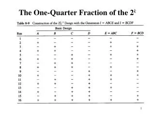
The One-Quarter Fraction of the 2 k. The One-Quarter Fraction of the 2 6-2. Complete defining relation: I = ABCE = BCDF = ADEF. The One-Quarter Fraction of the 2 6-2. Uses of the alternate fractions E = ± ABC, F = ± BCD

E N D
The One-Quarter Fraction of the 26-2 Complete defining relation: I = ABCE = BCDF = ADEF
The One-Quarter Fraction of the 26-2 • Uses of the alternate fractions E = ±ABC, F = ±BCD • Projection of the design into subsets of the original six variables • Any subset of 4 factors of the original 6 variables that is not a word in the complete defining relation will result in a full factorial design • Any subset of 4 factors of the original 6 variables that is a word in the complete defining relation will result in a replicated one-half factorial design • Consider ABCD (full factorial) • Consider ABCE (replicated half fraction) • Consider ABCF (full factorial)
Design Matrix of Example 8-4 • Injection molding process with six factors
Large effects: A, B, and AB (Ockham’s razor) The process is sensitive to temperature (A) if the screw speed (B) is at the high level => both A and B should be at the low level (reduce mean shrinkage) How about the part-to-part variability?
ŷ = bo + b1x1 + b2x2 + b12x1x2 = 27.3125 + 6.9375x1 + 17.8125x2 + 5.9375x1x2 e = y - ŷ
Residual plots indicate there are some dispersion effects, which can be quantified by an analysis of residuals.
Example 8-4 Factor C has a large dispersion effect. Its location effect is not large, so its level can be set to low to reduce variation.
Projection onto a cube in A, B, and C (Example 8-4) 26-2 -> 23 (n=2) B=low results in low values of average part shrinkage C=low produces low part-to-part variation => B-C- 10