Solving Large Markov Decision Processes
Solving Large Markov Decision Processes. Yilan Gu Dept. of Computer Science University of Toronto April 12, 2004. Outline. Introduction: what’s the problem ? Temporal abstraction Logical representation of MDPs Potential future directions. Markov Decision Processes (MDPs).

Solving Large Markov Decision Processes
E N D
Presentation Transcript
Solving Large Markov Decision Processes Yilan Gu Dept. of Computer Science University of Toronto April 12, 2004
Outline • Introduction: what’s the problem ? • Temporal abstraction • Logical representation of MDPs • Potential future directions
Markov Decision Processes (MDPs) • Decision-theoretic planning and learning problems are often modeled in MDPs. • An MDP is a model M = < S, A, T, R > consisting • a set of environment states S, • a set of actions A, • a transition function T: S A S [0,1] T(s,a,s’) = Pr (s’| s,a), • a reward function R: S A R . • A policy is a function : S A. • Expected cumulative reward -- value function V: S R . The Bellman Eq.: V(s) = R(s, (s)) + s’T(s, (s),s’) V(s’)
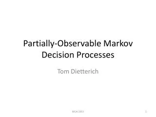
MDP Example 1 2 3 4 5 6 7 8 S = {(1,1), (1,2), …,(8,8)} A = {up, down, left, right} e.g., T((2,2),up,(1,2)) = 0.8, T((2,2),up,(2,1))=0.1, T((2,2),up,(2,3)) = 0.1, T((2,2),up,s’) = 0 for s’(1,2), (2,1), (2,3) …… R((1,8)) = 1, R(s)= -1 for s (1,8). +1 1 2 3 4 5 6 7 8 0.8 up (2,2) 0.1 0.1 Fig. The 8*8 grid world Notice: explicit representation of the model
Conventional Solution Algorithms for MDPs • Goal: looking for optimal policy * so that V*(s) = V*(s) V(s) for all sS and • Conventionalalgorithms • Dynamic programming: value iteration and policy iteration, • Decision tree search algorithm, etc. • Example: Value iteration Beginning with arbitrary V0; In each iteration n>0: for every s S , Qn(s,a) := R(s, a) + s’T(s, a, s’) Vn-1 (s’) for any a; Vn(s) := max a Qn(s,a) ; When n , Vn(s) V*(s). • Problem: it does not scale up!
Solving Large MDPs (Part I) • Temporal abstraction approaches (basic idea) • Solving MDPs hierarchically • Using complex actions or subtasks to compress the scales of the state spaces • Representing and solving MDPs in a logical way (basic idea) • Logically representing environment features • Aggregating ‘similar’ states • Representing effect of actions compactly by using logical structures, and eliminating unaffected features during reasoning
Options (Macro-Actions) Example 1 2 3 4 5 6 7 8 • Partition {S1 , S2 , S3 ,S4 } • A macro-action -- a local policy i : Si A on region Si • E.g., EPer (S1) = {(3,5),(5,3)} • Discounted transition model Ti: Si {i} Eper(Si) [0,1] • Discounted reward model Ri: Si {i} R 1 2 3 4 5 6 7 8 S1
Abstract MDP M’= < S’, A’, T’, R’> • S ’= Eper(Si ), e.g., • {(4,3),(3,4),(5,3),(3,5),(6,4),(4,6), (5,6),(6,5)} . • A’= Ai , where Ai is a set of macro-actions • on region Si . • Transition model T’: S ’ A’ S ’ [0,1] • T’(s, i, s’) = Ti(s, i,s’) if s Si , s’ Eper(Si ); • T’(s, i, s’) = 0 otherwise. • Reward model R’: S ’ A’ R • R’(s, i ) = Ri(s, i ) for any s’ Eper(Si ).
Other Temporal Abstraction Approaches • Options [Sutton 1995; Singh, Sutton and Precup 1999] Macro-actions [Hauskrecht et al. 1998; Parr 1998] • Fixed policies • Hierarchical abstract machines (HAMs) [Parr and Russell 1997; Andre and Russell 2001,2002] • Finite controllers • MAXQ methods [Dietterich 1998, 2000] • Goal-oriented subtasks • Etc.
Solving Large MDPs (Part II) • Temporal abstraction approaches (basic idea) • Solving MDPs hierarchically • Using complex actions or subtasks to compress the scale of the state spaces • Representing and solving MDPs logically (basic idea) • Logically representing environment features • Aggregating ‘similar’ states • Representing effect of actions compactly by using logical structures, and eliminating unaffected features during reasoning
First-Order MDPs • Using the stochastic situation calculus to model decision-theoretic planning problems • Underlying model : first-order MDPs (FOMDPs) • Solving FOMDPs using symbolic dynamic programming
Stochastic Situation Calculus (I) • Using choice axioms to specify possible outcomes ni(x) of any stochastic actiona(x) Example:choice(delCoff(x),a) a = delCoffS(x) a = delCoffF(x) • Situations: S0 , do(a,s) • Fluents F(x,s) – modeling environment features compactly Examples:office(x,s), coffeeReq(x,s), holdingCoffee(s) • Basic action theory: • Using successor state axioms to describe the effect of the actions’ outcomes on each fluent coffeeReq(x,do(a,s)) coffeeReq(x,s) a = delCoffS(x)
Stochastic Situation Calculus (II) • Asserting probabilities (may be depended on conditions of current situation Example: prob(delCoffS(x), delCoff(x), s) = case [hot, 0.9; hot, 0.7] • Specifying rewards/costs conditionally Example:R(do(a,s)) = case[ x. a = delCoffS(x) , 10; x.a = delCoffS(x) , 0] • stGolog programs, policies proc (x) if holdingCoffee then getCoffee else ( ?(coffeeReq(x)) ; delCoffee(x)) end proc
Symbolic Dynamic Programming • Representing value function Vn-1(s) logically case [1 (s) ,v1 ; … ; m (s) ,vm ] • Input: the system described in stochastic SitCal and Vn-1(s) • Output (also in case format): • Q-functions Q n(a(x),s)= R(s)+ iprob(ni(x),a(x),s) Vn-1(do(ni(x),s)) • Value function Vn(s) Vn(s) = ( a)( b) Q n(a,s) Q n(b,s)
Other Logical Representations • First-order MDPs [e.g., Boutilier et al. 2000; Boutilier, Reiter and Price 2001] • Factored MDPs [e.g., Boutilier and Dearden 1994, Boutilier, Dearden and Goldszmit 1995; Hoey et al. 1999] • Relational MDPs [e.g., Guestrin et al. 2003] • Integrated Bayesian Agent Language (IBAL) [Pfeffer 2001] • Etc [e.g., Bacchus 1993, Poole 1995].
Our Attempt: Combining temporal abstraction with logical representations of MDPs.
Motivation cityA cityB living(X, houseA) inCity(Y,cityA) houseB
Prior Work • MAXQ approaches [Dietterich 2000] and PHAMs method [Andre and Sutton 2001] • Using variables to represent state features • Propositional representations • Extending DTGolog with options [Ferrein, Fritz and Lakemeyer 2003] • Specifying options with the SitCal and Golog programs • Benefit: reusable when entering the exact same region • Shortage: options are based on explicit regions, and therefore not reusable under ‘similar’ regions
Our Idea and Potential Directions • Given any stGolog program (a macro-action schema) Example: proc getCoffee(X) if holdingCoffee then getCoffee else ( while coffeeReq(X) do delCoffee(X) ) end proc • Basic Idea – inspired by macro-actions [Boutilier et al 1998]: • Analyzing the macro-action to find what has been affected by the macro-action Example: holdingCoffee, coffeeReq(X) • Preprocessing discounted transition and reward models Example: tr(holdingCoffee coffeeReq(X) , getCoffee(X), holdingCoffee coffeeReq(X) )
(Continue) • using and re-using macro-actions as primitive actions • Benefit: • Schematic • Free variables in the macro-actions can represent a class of objects which have same characteristics • Even for infinite objects • Reusable in similar regions, other than the exact region
THE END Thank you!