Markov Decision Processes: A Survey
Markov Decision Processes: A Survey. Martin L. Puterman. Outline. Example - Airline Meal Planning MDP Overview and Applications Airline Meal Planning Models and Results MDP Theory and Computation Bayesian MDPs and Censored Models Reinforcement Learning Concluding Remarks.

Markov Decision Processes: A Survey
E N D
Presentation Transcript
Markov Decision Processes:A Survey Martin L. Puterman
Outline • Example - Airline Meal Planning • MDP Overview and Applications • Airline Meal Planning Models and Results • MDP Theory and Computation • Bayesian MDPs and Censored Models • Reinforcement Learning • Concluding Remarks Martin L. Puterman - June 2002
Airline Meal Planning • Goal: Get the right number of meals on each flight • Why is this hard? • Meal preparation lead times • Load uncertainty • Last minute uploading capacity constraints • Why is this important to an airline? • 500 flights per day 365 days $5/meal = $912,500 Martin L. Puterman - June 2002
Frequency -20 -10 0 10 20 30 Provisioning Error (Meals) How Significant is the Problem? Martin L. Puterman - June 2002
The Meal Planning Decision Process • At several key decision points up to 3 hours before departure, the meal planner observes reservations and meals allocated and adjusts allocated meal quantity. • Hourly in the last three hours, adjustments are made but the cost of adjustment is significantly higher and limited by delivery van capacity and uploading logistics. Martin L. Puterman - June 2002
18 hours Schedule, Production 6 hours Order Assembly 3 hours Order ready to go Departure Observe Passenger Load Delivery of Order Adjustments with Van Meal Planning Timeline Martin L. Puterman - June 2002
Airline Meal Planning • Operational goal; develop a meal planning strategy that minimizes expected total overage, underage and operational costs A Meal Planning Strategy specifies at each decision point the number of extra meals to prepare or deliver for any observed meal allocation and reservation quantity. Martin L. Puterman - June 2002
Why is Finding an Optimal Meal Planning Strategy Challenging? • 6 decision points • 108 passengers • 108 possible actions • One strategy requires 1081086 = 69984 order quantities. • There are 7,558,272 strategies to consider. • Demand must be forecasted. Martin L. Puterman - June 2002
Airline Meal Planning Characteristics • A similar decision is made at several time points • There are costs associated with each decision • The decision has future consequences • The overall cost depends on several events • There is uncertainty about the future Martin L. Puterman - June 2002
What is a Markov decision process? • A mathematical representation of a sequential decision making problem in which: • A system evolves through time. • A decision maker controls it by taking actions at pre-specified points of time. • Actions incur immediate costs or accrue immediate rewards and affect the subsequent system state. Martin L. Puterman - June 2002
MDP Overview Martin L. Puterman - June 2002
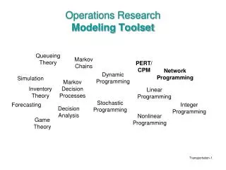
Markov Decision Processes are also known as: • MDPs • Dynamic Programs • Stochastic Dynamic Programs • Sequential Decision Processes • Stochastic Control Problems Martin L. Puterman - June 2002
Early Historical Perspective • Massé - Reservoir Control (1940’s ) • Wald - Sequential Analysis (1940’s ) • Bellman - Dynamic Programing (1950’s) • Arrow, Dvorestsky, Wolfowitz, Kiefer, Karlin - Inventory (1950’s) • Howard (1960) - Finite State and Action Models • Blackwell (1962) - Theoretical Foundation • Derman, Ross, Denardo, Veinott (1960’s) - Theory - USA • Dynkin, Krylov, Shirayev, Yushkevitch (1960’s) - Theory - USSR Martin L. Puterman - June 2002
Basic Model Ingredients • Decision epochs – {0, 1, 2, …., N} or [0,N] or {0,1,2, …} or [0,) • State Space – S (generic state s) • Action Sets – As (generic action a) • Rewards – rt(s,a) • Transition probabilities – pt(j|s,a) A model is called stationary if rewards and transition probabilities are independent of t Martin L. Puterman - June 2002
System Evolution at+1 at st st+1 rt(st,at) rt+1(st+1,at+1) Decision Epoch t +1 Decision Epoch t Martin L. Puterman - June 2002
Another Perspective s1 s1 a1 s2 s2 s3 s3 a2 s4 s4 Martin L. Puterman - June 2002
Yet Another Perspective:An Event Timeline ... May 15 June 1 June 10 June 15 ... Place June order May order arrives; ship product to DCs May sales data arrives; prepare July forecast Place July order Martin L. Puterman - June 2002
Some Variants on the Basic Model • There may be a continuum of states and/or actions • Decisions may be made in continuous time • Rewards and transition rates may change over time • System state may be not observable • Some model parameters may not be known Martin L. Puterman - June 2002
Derived Quantities • Decision Rules: dt(s) • Policies, Strategies or Plans: = ( d1, d2, …) or = ( d1, d2, …, dN) • Stochastic Processes : ( Xt, Yt ), Es { } • Value Functions: vt (s), v(s), g , … • Value functions differ from immediate rewards, they represent the value starting in a state of all future events Martin L. Puterman - June 2002
Objective Identify a policy that maximizes either the • expected total reward (finite or infinite horizon) v(s) = Es { rt (Xt,Yt ) } • expected discounted reward • expected long run average reward • expected utility possibly subject to constraints on system performance t=0 Martin L. Puterman - June 2002
The Bellman Equation • MDP computation and theory focuses on solving the optimality (Bellman) equation which for infinite horizon discounted models This can also be expressed as v = Tv or Bv = 0 v(s) is the value function of the MDP Martin L. Puterman - June 2002
Some Theoretical Issues • When does an optimal policy with nice structure exist? • Markov or Stationary Policy • (s,S) or Control Limit Policy • When do computational algorithms converge? and how fast? • What properties do solutions of the optimality equation have? Martin L. Puterman - June 2002
Computing Optimal Policies • Why? • Implementation • Gold Standard for Heuristics • Basic Principle - Transform multi-period problem into a sequence of one-period problems. • Why is computation difficult in practice? • Curse of Dimensionality Martin L. Puterman - June 2002
Computational Methods • Finite Horizon Models • Backward Induction (Dynamic Programming) • Infinite Horizon Models • Value Iteration • Policy Iteration • Modified Policy Iteration • Linear Programming • Neuro-Dynamic Programming/Reinforcement learning Martin L. Puterman - June 2002
Infinite Horizon Computation ~ • Iterative algorithms work as follows: • Approximate the value function by v(s) • Select a new decision rule by • Re-approximate the value function • Approximation methods • exact - policy iteration • iterative - value iteration and modified policy iteration • simulation based - reinforcement learning Martin L. Puterman - June 2002
Airline Meal Planning Behaviourial Ecology Capacity Expansion Decision Analysis Equipment Replacement Fisheries Management Gambling Systems Highway Pavement Repair Inventory Control Job Seeking Strategies Knapsack Problems Learning Medical Treatment Network Control Applications (A to N) Martin L. Puterman - June 2002
Option Pricing Project Selection Queueing System Control Robotic Motion Scheduling Tetris User Modeling Vision (Computer) Water Resources X-Ray Dosage Yield Management Zebra Hunting Applications (O to Z) Martin L. Puterman - June 2002
“Coffee, Tea or …? A Markov Decision Process Model for Airline Meal Provisioning” J. Goto, M.E. Lewis and MLP • Decision Epochs: T= {1, …,5} • 0 - Departure time • 1-3: 1,2 and 3 Hours Pre-Departure • 4: 6 Hours Pre - Departure • 5: 36 Hours Pre-Departure • States: {(l,q): 0 l Booking Limit, 0 q Capacity} • Actions: (Meal quantity after delivery) • At,(l,q)= { 0, 1, …, Plane Capacity} t = 3,4,5 • At,(l,q) = {q-van capacity, …, q + van capacity) t= 1,2 Martin L. Puterman - June 2002
Markov Decision Process Formulation Costs: (depending on t) rt((l,q),a) = Meal Cost + Return penalty + late delivery charge + shortage cost Transition Probabilities: pt(q’|q) a=q’ pt((l’,q’)|(l,q),a) = 0 aq’ Martin L. Puterman - June 2002
18 hours Schedule, Production 6 hours Order Assembly 3 hours Order ready to go An Optimal Decision Rule Meal Quantity Decision Epoch 1 Passenger Load Departure Adjust with Van Martin L. Puterman - June 2002
Actual Mean = 9.81 Standard Deviation = 8.46 Frequency Model (out of sample) Mean = 7.99 Standard Deviation = 6.96 Frequency -20 0 20 40 Provisioning Error Empirical Performance Martin L. Puterman - June 2002
Overage versus Shortage • Evaluate the model over a range of terminal costs • Observe the relationship of average overage and proportion of flights short-catered • 55 flight number / aircraft capacity combinations (evaluated separately) Martin L. Puterman - June 2002
Overage versus Shortage Performance of optimal policies Martin L. Puterman - June 2002
Information Acquisition Martin L. Puterman - June 2002
Objective: Investigate the tradeoff between acquiring information and optimal policy choice Examples: Harpaz, Lee and Winkler (1982) study output decisions of a competitive firm in a market with random demand in which the demand distribution is unknown. Braden and Oren (1994) study dynamic pricing decisions of a firm in a market with unknown consumer demand curves. Lariviere and Porteus (1999) and Ding, Puterman and Bisi (2002) study order decisions of a censored newsvendor with unobservable lost sales and unknown demand distributions. Key result - it is optimal to “experiment” Information Acquisition and Optimization Martin L. Puterman - June 2002
Bayesian Newsvendor Model • Newsvendor cost structure (c - cost, h - salvage value, p - penalty cost) • Demand assumptions • positive continuous • i.i.d. sample from f(x|) with unknown • prior on is 1() • Assume first that demand is unobservable Demand = Sales + “observed” lost sales Martin L. Puterman - June 2002
Time Line of Events obs. x1 set y2 obs. x2 set y1 1 2 3 Martin L. Puterman - June 2002
Demand Updating xn n n+1 Martin L. Puterman - June 2002
Bayesian Newsvendor Model Bayesian MDP Formulation At decision epoch n, (n=1,2, ..., N) • States: {all probability distributions on the unknown parameter} • Actions: • Costs: • Transition Prob: Martin L. Puterman - June 2002
Bayesian Newsvendor Model The Optimality Equations for n=1,…,N with the boundary condition: Key Observation The transition probabilities are independent of the actions. So the problem can be reduced to a sequence of single-period problems. Martin L. Puterman - June 2002
xn-1 The Bayesian Newsvendor Policy The BMDP reduces to a sequence of single-period, two-step problems. • Demand distribution parameter updating • Cost minimization where Mn is the CDF of mn Martin L. Puterman - June 2002
Bayesian Newsvendor with Unobservable Lost Sales • Model Set-up • Same as fully observable case but unmet demand is lost and unobservable • Question • Is the Bayesian Newsvendor policy optimal? Martin L. Puterman - June 2002
Demand is censored by the order quantity. : demand exactly observed : demand censored Demand updating is different in this case: Bayesian Newsvendor with Unobservable Lost Sales Martin L. Puterman - June 2002
Bayesian Newsvendor with Unobservable Lost Sales obs. xn-1=0 with mn-1(0) Set yn-1 obs. xn-1=1 with mn-1(1) obs. xn-1 = yn-1with[1-Mn-1(yn-1)] Martin L. Puterman - June 2002
Bayesian Newsvendor with Unobservable Lost Sales Model Formulation • States, Actions, Costs: As above • Transition Probabilities: The Optimality Equations Martin L. Puterman - June 2002
Bayesian Newsvendor with Unobservable Lost Sales The Key Result • if f(x| ) is likelihood order increasing in . • In this model, decisions in separate periods are interrelated through the optimality equation. • This means that it is optimal to tradeoff learning for short term optimality. • Question: What is an upper bound on yn*? Martin L. Puterman - June 2002
Bayesian Newsvendor with Unobservable Lost Sales • Solving the optimality equations gives • For N: • For n=1,..., N-1, where p’(yn) is a “policy dependent penalty cost . Proof of key result is based on showing p’(yn) > p for n < N. Martin L. Puterman - June 2002
Bayesian Newsvendor with Unobservable Lost Sales • Some comments • The extra penalty can be interpreted as the marginal expected value of information at decision epoch n. • Numerical results show small improvements when using the optimal policy as opposed to the Bayesian Newsvendor policy. • We have extended this to a two level supply chain Martin L. Puterman - June 2002
Partially Observed MDPs • In POMDPs, system state is not observable. • Decision maker receives a signal y which is related to the system state by q(y|s,a). • Analysis is based on using Bayes Theorem to estimate distribution of the system state given the signal • Similar to Bayesian MDPs described above • the posterior state distribution is a sufficient statistic for decision making • State space is a continuum • Early work by Smallwood and Sondik (1972) • Applications • Medical diagnosis and treatment • Equipment repair Martin L. Puterman - June 2002