Download
1 / 26
260 likes | 279 Vues
This approach relies on known circuit form to find constants using basic tools, skipping differential equations. Learn to analyze circuits with one energy storing element using Thevenin circuits. Obtain the time constant and determine the variables step by step.

E N D
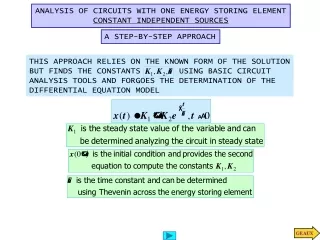
THIS APPROACH RELIES ON THE KNOWN FORM OF THE SOLUTION BUT FINDS THE CONSTANTS USING BASIC CIRCUIT ANALYSIS TOOLS AND FORGOES THE DETERMINATION OF THE DIFFERENTIAL EQUATION MODEL ANALYSIS OF CIRCUITS WITH ONE ENERGY STORING ELEMENT CONSTANT INDEPENDENT SOURCES A STEP-BY-STEP APPROACH
Thevenin CIRCUITS WITH ONE ENERGY STORING ELEMENT • Obtaining the time constant: A General Approach Use KVL KCL@ node a
STEP 1. THE FORM OF THE SOLUTION STEP 2: DRAW THE CIRCUIT IN STEADY STATE PRIOR TO THE SWITCHING AND DETERMINE CAPACITOR VOLTAGE OR INDUCTOR CURRENT STEP 3: DRAW THE CIRCUIT AT 0+ THE CAPACITOR ACTS AS A VOLTAGE SOURCE. THE INDUCTOR ACTS AS A CURRENT SOURCE. DETERMINE THE VARIABLE AT t=0+ THE STEPS STEP 5: DETERMINE THE TIME CONSTANT STEP 6: DETERMINE THE CONSTANTS K1, K2 STEP 4: DRAW THE CIRCUIT IN STEADY STATE AFTER THE SWITCHING AND DETERMINE THE VARIABLE IN STEADY STATE.
KVL LEARNING EXAMPLE USE A CIRCUIT VALID FOR t=0+. THE CAPACITOR ACTS AS SOURCE USE CIRCUIT IN STEADY STATE PRIOR TO THE SWITCHING NOTES FOR INDUCTIVE CIRCUIT (1)DETERMINE INITIAL INDUCTOR CURRENT IN STEP 2 (2)FOR THE t=0+ CIRCUIT REPLACE INDUCTOR BY A CURRENT SOURCE
ORIGINAL CIRCUIT NOTE: FOR INDUCTIVE CIRCUIT USE CIRCUIT IN STEADY STATE AFTER SWITCHING
USING MATLAB TO DISPLAY FINAL ANSWER Command used to define linearly spaced arrays » help linspace LINSPACE Linearly spaced vector. LINSPACE(x1, x2) generates a row vector of 100 linearly equally spaced points between x1 and x2. LINSPACE(x1, x2, N) generates N points between x1 and x2. See also LOGSPACE, :. Script (m-file) with commands used. Prepared with the MATLAB Editor %example6p3.m %commands used to display funtion i(t) %this is an example of MATLAB script or M-file %must be stored in a text file with extension ".m” %the commands are executed when the name of the M-file is typed at the %MATLAB prompt (without the extension) tau=0.15; %define time constant tini=-4*tau; %select left starting point tend=10*tau; %define right end point tminus=linspace(tini,0,100); %use 100 points for t<=0 tplus=linspace(0,tend, 250); % and 250 for t>=0 iminus=2*ones(size(tminus)); %define i for t<=0 iplus=36/8+5/6*exp(-tplus/tau); %define i for t>=0 plot(tminus,iminus,'ro',tplus,iplus,'bd'), grid; %basic plot command specifying %color and marker title('VARIATION OF CURRENT i(t)'), xlabel('time(s)'), ylabel('i(t)(mA)') legend('prior to switching', 'after switching') axis([-0.5,1.5,1.5,6]);%define scales for axis [xmin,xmax,ymin,ymax]
LEARNING EXAMPLE Use circuit at t=0+. Inductor is replaced by current source Use circuit in steady state prior to switching
USE CIRCUIT IN STEADY STATE AFTER SWITCHING ORIGINAL CIRCUIT
OPEN CIRCUIT VOLTAGE KVL KVL ORIGINAL CIRCUIT
SHORT CIRCUIT CURRENT NOTE: FOR THE INDUCTIVE CASE THE CIRCUIT USED TO COMPUTE THE SHORT CIRCUIT CURRENT IS THE SAME USE TO DETERMINE ORIGINAL CIRCUIT
KVL LEARNING EXTENSION
KVL ORIGINAL CIRCUIT OPEN CIRCUIT VOLTAGE SHORT CIRCUIT CURRENT
Inductor example STEP 2: Initial inductor current STEP 3: Determine output at 0+ (inductor current is constant) STEP 1: Form of the solution
Step by Step Pulse Response STEP 4: Find output in steady state after the switching STEP 6: Find the solution STEP 5: Find time constant after switch
PULSE RESPONSE WE STUDY THE RESPONSE OF CIRCUITS TO A SPECIAL CLASS OF SINGULARITY FUNCTIONS VOLTAGE STEP CURRENT STEP TIME SHIFTED STEP
LEARN BY DOING PULSE SIGNAL PULSE AS SUM OF STEPS
RESPONSE FOR CONSTANT SOURCES NONZERO INITIAL TIME AND REPEATED SWITCHING This expression will hold on ANY interval where the sources are constant. The values of the constants may be different and must be evaluated for each interval The values at the end of one interval will serve as initial conditions for the next interval
THE SWITCH IS INITIALLY AT a. AT TIME t=0 IT MOVES TO b AND AT t=0.5 IT MOVES BACK TO a. FIND Piecewise constant source EXAMPLE The constants are determined in the usual manner
USING MATLAB TO DISPLAY OUTPUT VOLTAGE First Order %pulse1.m % displays the response to a pulse response tmin=linspace(-0.5,0,50); %negative time segment t1=linspace(0,0.5,50); %first segment t2=linspace(0.5, 1.5,100); %second segment vomin=12*ones(size(tmin)); vo1=12*exp(-t1/0.2); %after first switching vo2=12-11.015*exp(-(t2-0.5)/0.2); %after second switching plot(tmin,vomin,'bo',t1,vo1,'rx',t2,vo2,'md'),grid title('OUTPUT VOLTAGE'), xlabel('t(s)'),ylabel('Vo(V)')