Iterated Integrals | Mastering Double Integrals
E N D
Presentation Transcript
15 MULTIPLE INTEGRALS
MULTIPLE INTEGRALS • Recall that it is usually difficult to evaluate single integrals directly from the definition of an integral. • However, the Fundamental Theorem of Calculus (FTC) provides a much easier method.
MULTIPLE INTEGRALS • The evaluation of double integrals from first principles is even more difficult.
MULTIPLE INTEGRALS 15.2 Iterated Integrals • In this section, we will learn how to: • Express double integrals as iterated integrals.
INTRODUCTION • Once we have expressed a double integral as an iterated integral, we can then evaluate it by calculating two single integrals.
INTRODUCTION • Suppose that f is a function of two variables that is integrable on the rectangle R = [a, b] x [c, d]
INTRODUCTION • We use the notation to mean: • x is held fixed • f(x, y) is integrated with respect to yfrom y = c to y = d
PARTIAL INTEGRATION • This procedure is called partial integration with respect to y. • Notice its similarity to partial differentiation.
PARTIAL INTEGRATION • Now, is a number that depends on the value of x. • So,it defines a function of x:
PARTIAL INTEGRATION Equation 1 • If we now integrate the function Awith respect to x from x = a to x = b, we get:
ITERATED INTEGRAL • The integral on the right side of Equation 1 is called an iterated integral. • Usually, the brackets are omitted.
ITERATED INTEGRALS Equation 2 • Thus, means that: • First, we integrate with respect to y from c to d. • Then, we integratewith respect to x from a to b.
ITERATED INTEGRALS • Similarly, the iterated integralmeans that: • First, we integrate with respect to x (holding y fixed) from x = a to x = b. • Then, weintegrate the resulting function of ywith respect to y from y = c to y = d.
ITERATED INTEGRALS • Notice that, in both Equations 2 and 3, we work from the inside out.
ITERATED INTEGRALS Example 1 • Evaluate the iterated integrals. • a. • b.
ITERATED INTEGRALS Example 1 a • Regarding x as a constant, we obtain:
ITERATED INTEGRALS Example 1 a • Thus, the function A in the preceding discussion is given by in this example.
ITERATED INTEGRALS Example 1 a • We now integrate this function of xfrom 0 to 3:
ITERATED INTEGRALS Example 1 b • Here, we first integrate with respect to x:
ITERATED INTEGRALS • Notice that, in Example 1, we obtained the same answer whether we integrated with respect to y or x first.
ITERATED INTEGRALS • In general, it turns out (see Theorem 4) that the two iterated integrals in Equations 2 and 3 are always equal. • That is, the order of integration does not matter. • This is similar to Clairaut’s Theorem on the equality of the mixed partial derivatives.
ITERATED INTEGRALS • The following theorem gives a practical method for evaluating a double integral by expressing it as an iterated integral (in either order).
FUBUNI’S THEOREM Theorem 4 • If f is continuous on the rectangle R = {(x, y) |a≤ x ≤ b, c≤ y ≤ dthen
FUBUNI’S THEOREM Theorem 4 • More generally, this is true if we assume that: • f is bounded on R. • f is discontinuous only on a finite number of smooth curves. • The iterated integrals exist.
FUBUNI’S THEOREM • Theorem 4 is named after the Italian mathematician Guido Fubini (1879–1943), who proved a very general version of this theorem in 1907. • However, the version for continuous functions was known to the French mathematician Augustin-Louis Cauchy almost a century earlier.
FUBUNI’S THEOREM • The proof of Fubini’s Theorem is too difficult to include in this book. • However, we can at least give an intuitive indication of why it is true for the case where f(x, y) ≥ 0.
FUBUNI’S THEOREM • Recall that, if f is positive, then we can interpret the double integral as: • The volume V of the solid S that lies above R and under the surface z = f(x, y).
FUBUNI’S THEOREM • However, we have another formula that we used for volume in Chapter 6, namely,where: • A(x) is the area of a cross-section of S in the plane through x perpendicular to the x-axis.
FUBUNI’S THEOREM • From the figure, you can see that A(x) is the area under the curve C whose equation is z = f(x, y) where: • x is held constant • c≤ y ≤ d
FUBUNI’S THEOREM • Therefore,Then, we have:
FUBUNI’S THEOREM • A similar argument, using cross-sections perpendicular to the y-axis, shows that:
FUBUNI’S THEOREM Example 2 • Evaluate the double integral where R = {(x, y)| 0 ≤ x ≤ 2, 1 ≤ y ≤ 2} • Compare with Example 3 in Section 15.1
FUBUNI’S THEOREM E. g. 2—Solution 1 • Fubini’s Theorem gives:
FUBUNI’S THEOREM E. g. 2—Solution 2 • This time, we first integrate with respect to x:
FUBUNI’S THEOREM • Notice the negative answer in Example 2. • Nothing is wrong with that. • The function f in the example is not a positive function. • So, its integral doesn’t represent a volume.
FUBUNI’S THEOREM • From the figure, we see that f is always negative on R. • Thus, thevalue of the integral is the negative of the volume that lies above the graph of f and below R.
ITERATED INTEGRALS Example 3 • Evaluate where R = [1, 2] x [0, π]
ITERATED INTEGRALS E. g. 3—Solution 1 • If we first integrate with respect to x, we get:
ITERATED INTEGRALS E. g. 3—Solution 2 • If we reverse the order of integration, we get:
ITERATED INTEGRALS E. g. 3—Solution 2 • To evaluate the inner integral, we use integration by parts with:
ITERATED INTEGRALS E. g. 3—Solution 2 • Thus,
ITERATED INTEGRALS E. g. 3—Solution 2 • If we now integrate the first term by parts with u = –1/x and dv = π cos πxdx, we get: du = dx/x2v = sin πx and
ITERATED INTEGRALS E. g. 3—Solution 2 • Therefore, • Thus,
ITERATED INTEGRALS • In Example 2, Solutions 1 and 2 are equally straightforward. • However, in Example 3, the first solution is much easier than the second one. • Thus, when we evaluate double integrals, it is wise to choose the order of integration that gives simpler integrals.
ITERATED INTEGRALS Example 4 • Find the volume of the solid S that is bounded by: • The elliptic paraboloid x2 + 2y2 + z = 16 • The planes x = 2 and y = 2 • The three coordinate planes
ITERATED INTEGRALS Example 4 • We first observe that S is the solid that lies: • Under the surface z = 16 – x2 – 2y2 • Above the square R = [0, 2] x [0, 2]
ITERATED INTEGRALS Example 4 • This solid was considered in Example 1 in Section 15.1. • Now, however, we are in a position to evaluate the double integral using Fubini’s Theorem.
ITERATED INTEGRALS Example 4 • Thus,
ITERATED INTEGRALS • Consider the special case where f(x, y) can be factored as the product of a function of x only and a function of y only. • Then, the double integral of f can be written in a particularly simple form.
ITERATED INTEGRALS • To be specific, suppose that: • f(x, y) = g(x)h(y) • R = [a, b] x [c, d]