Measurement Techniques for Accelerator Lattice Parameters: An Overview
This lecture offers an introduction to the most commonly used methods for measuring key parameters of accelerator lattices. Key parameters include the dispersion function, Twiss parameters, and beta functions, which are essential for understanding machine performance impacts like brightness and luminosity. The presentation discusses how lattice measurements can deviate from design due to various errors and highlights the iterative correction process necessary for optimizing lattice parameters. It covers techniques for measuring dispersion, Twiss parameters, and response to dipole kicks.

Measurement Techniques for Accelerator Lattice Parameters: An Overview
E N D
Presentation Transcript
Lattice Measurement JörgWenninger CERN Accelerators and Beams Department Operations group May 2008 Acknowledgements : A. S. Müller, P. Castro CERN Accelerator School : Beam Diagnostics, 28 May - 6 June 2008, Dourdan, France
Introduction / I • This lecture is an introduction to the most commonly used methods to measure the key parameters of an accelerator lattice. • The lattice parameters that will be covered are : • Dispersion function • Twiss parameters: • Betatron function b, • Phase advance m, • Betatron function dericative a = (1+db/ds)/2. The errors on b and m are frequently referred to as beta-beatingand phase-beating
Introduction / II • The knowledge of the lattice parameters is essential since they have a strong influence on machine performance: • Beam envelope : brightness, luminosity, aperture, emittance growth during transfer .... • Stability & lifetime (resonances...) • ... • The actual lattice may deviate from the design lattice due to a variety of errors (magnet transfer functions, control system errors... ). • In general the measurements are followed a by second step : the correction of the measured lattice errors. This is frequently an iterative process that is repeated until the lattice parameters are judged to be satisfactory.
Dispersion Definition • The dispersion function Du(s) defines the local sensitivity of the beam trajectory or orbit u(s) to a relative energy error dp/p: • Non-zero dispersion is produced by bending magnets (or any dipole kick). • A perfectly straight transfer line (linear accelerator) has Dx = Dy = 0. • For a planar ring, Dx 0, Dy = 0. • In a ‚real‘ ring, non-zero vertical dispersion may be produced by coupling (xy) or by vertical misalignments of the accelerator elements, in particular quadrupoles.
Dispersion Measurement The dispersion function is the lattice parameter that is easiest to measure. Based on its definition one has to measure the orbit/trajectory for different values of dp/p. The simplest way to induce an energy shift is to change the RF frequency For synchrotron light sources, the factor g2 can normally be neglected. This is usually not the case for protons, except for very high energy (like LHC). • ac = momentum compaction factor • = E/m gt = g value at transition
Dispersion Measurement : Ring • Dispersion measured in the CERN SPS ring (protons 14 to 450 GeV/c) for the horizontal plane. • SPS has a simple ~90 lattice. • 6 long straight sections with low horizontal dispersion.
Dispersion Measurement : Transfer Line • Dispersion measured in a transfer line, here the 400 GeV/c high intensity proton transfer line from the SPS ring to the CERN Neutrino to Gran Sasso target. • The transfer line bends both horizontally and vertically. • The dispersion is matched to be 0 at the target. • The dispersion is obtained by varying the RF frequency in the SPS ring and measuring the trajectory for different SPS RF frequency settings. SPS ring Vertical • Model • Data fit • Data Target Horizontal
K-modulation • When the strength K0 of a selected quadrupole (length L) in a ring is changed by a small amount DK, the associated tune change DQ is : • This relation may be used to determine the average betatron function if: • The selected quadrupole is individually powered. • The strength change DK is (sufficiently) well known: • Magnet tranfer function & hysteresis. • For long magnets, resp. when b changes significantly over the length of the magnet, it is necessary to integrate numerically. • The tune can be measured with high accuracy – for example with a PLL. • A very elegant way is to modulate the strength in time at a frequency f, for example • and detect the frequency of the oscillation. In that case more than one magnet can be measured at the same time, provided the DK‘s are small enough. >> directly prop. to b !!!
K-modulation Example • Example of the period tune modulation due to the modulation of a LEP quadrupole (here with a square function). O. Berrig et al, DIPAC01
Response to Dipole Kicks The orbit or trajectory response matrix relates the position change at monitors to the deflection at steering magnets (usually orbit correctors). The position change Dui at the ith monitor is related to a kick qj at the jth corrector by : R = response matrix In a linear approximation : Closed orbit Optics information is ‘entangled’ in R Trajectory
Response : remarks… • R does not provide direct information on the optical function b, m, …: • Step 1: the model must be adjusted (fit) to match the measured R. • Step 2 : the optical functions are obtained from the matched model. • In a transfer line the optical functions depend on the initial conditions. The R matrix seems to give information on b etc, but in reality it does not ! It only provides information on the correctness of the line settings. • The measured R also depends on the BPM and corrector calibrations: • complicates fits, the C’s may depend on amplitude ! • R is not limited to linear effects, at large enough amplitudes non-linear effect can potentially be observed. Coupling may be included in the data fit.
Fitting Response Data • To extract information from response data, it is necessary to compare the model matrix with the measured matrix: • The number of fit parameters ci can be very large : • BPM calibration factors • Corrector calibration factors • Quadrupole strengths • etc • >> for a large ring : • the number of elements (NxM) can easily exceed 10’000 ! • the number of parameters n can easily reach ~ 1000 ! number elements : N monitors x M correctors Parameter vector :
Response Fits : Technique /1 • Data preparation : • We build a vector r holding the weighted difference between the measured and modeled response for all matrix elements : s is the measurement error 2) Local gradient : We must now evaluate the sensitivity of each element of r with respect our parameters ci. The gradients may be represented by a matrix G. For quadrupole gradients or other complex parameters, it may be necessary to compute the gradient numerically by computing R for ci and for ci.+Dci.
Response Fits : Technique /2 3) Least-square minimization : Try to find the increments to the parameters that minimize the difference between data and model. To this end we must solve the linearised equation for parameter changes Dc: 4) Iteration : Update c, update G, solve again… until the solution is stable. m = # elements Rij If the errors are distributed according to a gaussian distribution and if the fit is good, then the residual converges towards m-n.
‘LOCO’ There are many versions of response fits available at various laboratories. A popular version is LOCO (Linear Optics from Closed Orbits), written initially in FORTRAN by J. Safranek, which in the meantime exists also as Mathlab version. G. Portman et al, Beam Dynamics Newsletter No. 44
LOCO Results Example of the optics of the VUV ring at NSLS before (left) and after (right) measurement and correction of the optics using LOCO. J. Safranek, Beam Dynamics Newsletter No. 44
Transfer Line Example • Initial measurement : • First Hor corrector data does not fit the line model at all !! • >> Perform a fit with quadrupole strengths as free parameters. The fit indicates that one quadrupole is too weak by 20% ! Second measurement : After correction of the quadrupole strength model and data fit. Histogram : data *+ Line : model fit
Phase Advance Measurement The betatron oscillation of a bunch measured turn by turn in a ring at a BPM number i can be expressed as: • k = turn number • A(k) = amplitude at turn k • = phase factor • Q = tune Example of a damped betatron oscillation following a kick y = overall phase factor for all BPMs The difference of the phase factors for 2 BPMs is nothing but the betatron phase advance Dm = mi-mj: >> Direct measurement of the betatron phase advance
Twiss Parameter Reconstruction • The phase advance may be reconstructed with high accuracy using a Fourier Transform provided • the betatron oscillation is long enough (damping !). • the turn-by-turn resolution of the BPMs is good. • >> results do not depend on the BPM calibration !! • The betatron function may be reconstructed at any BPM using the measured phase advance to 2 adjacent BPMs: • Attention : • Model information is used to reconstruct b !! • The accuracy on b depends on potential sources of errors within the region. • Unless the error is huge, this introduced only a small error (~%) on the reconstructed b. 1 2 3 Dm12 Dm23
Betatron Function Reconstruction • Example for an online reconstruction of the horizontal betatron function (top) and betatron beating (bottom, bmeas/bmodel) for a LEP arc. • b,m, and a may be reconstructed by interpolations (based on the model) for all elements located within the region of a BPM triplet. P. Castro, PAC91
LEP 45 GeV Optics • Example of measured beta-beating at LEP (45 GeV) • The largest step in beta-beating occur near the interaction points (IP) at the low beta insertions. P. Castro, PHD
Measurement Errors The error on the reconstructed b value is given for ‘equidistant’ BPMs by : • The error depends on: • The error on the phase sf. • For long oscillations / good BPMs an error of less than 1 can be obtained. • The phase advance Dm. sf = 0.5 >> The error increases dramatically when Dm approaches 90 Dm
Beta-beating and 90 Phase Advance The b-beating induced by a gradient error DK due to an element of length L located at position s0 is: >> The b-beat phase advances at twice the betatron phase ! For BPMs with Dm = 90 the b-beat wave phase advances by 180 : >> At the Nyquist frequency – impossible to measure the amplitude of the b-beat wave Illustration : depending on the phase of the b-beat wave, the BPMs measure a different amplitude – anything from 0 to the right value ! 180
Beam Exciters Classical ‘exciter’ : ‘Kicker’ magnet Advanced ‘exciter’ : AC dipole • Forced oscillation. • Provides long oscillation periods. • Frequency close to Q, but sufficiently far away to avoid emittance blowup • ideal for protons & ions O. Berrig et al, DIPAC01
Fits Forever ! Fits are a great invention, and with the advent of powerful PCs, it is nowadays very easy to join the great fitters club. It is possible to build complicated fits that combined response, dispersion, phase advance etc.. The only limit is your imagination ! There are a few things to watch out when you are not yet an experienced ‚fitter‘ : Complicated fits like the response fits may be plagued with singularities that must be carefully removed or you may get non-sense: In LOCO singularities are removed by ‚eigenvalue‘ cuts. Before throwing thousands of parameters at your fit, start with a limited number and watch how the results change. Watch out for redundant fit parameters. For example : If you are trying to vary the strengths of multiple quadrupoles located between 2 BPMs, you may get non-sense because you have more parameters than constraints ! Checkout your fits with simulations including ‚realistic‘ errors and noise.
Summary My private rating !
K-modulation : BPM offsets K-modulation may also be used in parallel to measure the beam offset uQ in the modulated quadrupole, since the orbit change Du induced by the modulation is: The modulation amplitude at frequency f vanishes when the beam is centered in the quadrupole uQ = 0>> determine measurement offset of the BPMs. uQ uQ f ~ hew Hz (or less)