Regression Analysis and Variable Transformations: Enhancing Statistical Accuracy
Learn how to include dummy variables and interaction effects in regression analysis, and the significance of variable transformations for accurate statistical representations. Explore examples and considerations for addressing common issues in data analysis.

Regression Analysis and Variable Transformations: Enhancing Statistical Accuracy
E N D
Presentation Transcript
University of Warwick, Department of Sociology, 2012/13SO 201: SSAASS (Surveys and Statistics) (Richard Lampard)Week 6Regression: ‘Loose Ends’
Dummy variables • Categorical variables can be included in regression analyses via the use of one or more dummy variables (two-category variables with values of 0 and 1). • In the case of a comparison of men and women, a dummy variable could compare men (coded 1) with women (coded 0).
Interaction effects… Women Length of residence All Men Age In this situation there is an interaction between the effects of age and of gender, so B (the slope) varies according to gender and is greater for women
Creating a variable to check for an interaction effect • We may want to see whether an effect varies according to the level of another variable. • Multiplying the values of two independent variables together, and including this third variable alongside the other two allows us to do this.
Interaction effects (continued) Women Length of residence Slope of line for women = BAGE All Men Slope of line for men = BAGE+BAGESEXD Age SEXDUMMY = 1 for men & 0 for women AGESEXD = AGE x SEXDUMMY For men AGESEXD = AGE & For women AGESEXD = 0
Transformations • There is quite a useful chapter on transformations in Marsh and Elliott (2009). • This makes the point that transformations can be applied to either one or more independent variables or the dependent variable within a regression analysis. • Transformations often take the form of raising a variable to a particular power (e.g. squaring it, cubing it, etc., and can take the inverse form of these too (e.g. taking its square root). • Logarithmic transformations are also fairly common, e.g. in relation to variables such as income.
Reasons for transformations • Transformations can lead to a more accurate representation of the form of the relationship between two variables. • But they can also sometimes resolve deviations from regression assumptions more generally!
An example These lengths of residence at current address relate to a sample of cases from the 1995 General Household Survey.
Some immediate problems • If we are using length of residence as the dependent variable in a regression analysis, then since the lengths of residence of individuals within households (e.g. members of couples) are likely to be related, and hence the residuals are likely not to be independent, one of the regression assumptions looks problematic. • We will also need to take account of (control for) age in some way, since this has obvious implications for length of residence. • But as the next slide shows, we might expect the diversity of lengths of residence to increase with increasing age, hence the assumption of homoscedasticity seems problematic too...
Line showing maximum possible length for a given age Length of residence Two-headed arrows show increasing scope for diversity Age
Outlier Length of Residence (y) B 1 ε C Age (x) 0 Regression line y = Bx + C + ε Error term (Residual) Slope Constant
Do the residuals have a normal distribution? The distribution of the residuals is, unsurprisingly, asymmetric. A One-Sample Kolmogorov-Smirnov test with a statistic of 6.864 shows it differs significantly from a normal distribution (p<0.001).
What happens if we add age2? It looks as if age-squared does a rather better job of representing the relationship than age does when they are included together! But how does that help us? A One-Sample Kolmogorov-Smirnov test with a statistic of 6.596 shows the distribution of residuals still differs significantly from a normal distribution (p<0.001)...
What if we take the square root of LoR rather than square age?
Are the residuals now closer to a normal distribution? The distribution of the residuals is now much more symmetric. But a One-Sample Kolmogorov-Smirnov test with a statistic of 1.503 shows it still differs significantly from a normal distribution (p=0.022).
Adding sex to the regression... Adding sex to the regression in the form of the dummy variable described earlier doesn’t seem to have achieved much...
But wait... Is there an interaction? ‘asd’ is the AGESEXD interaction term described earlier. Its effect is (just) significant: p=0.041 < 0.05 Meanwhile, the K-S statistic is now only just significant (1.373; p=0.046)
Adding a set of class dummies • SC1 is 1 for Class I, 0 otherwise • SC2 is 1 for Class II, 0 otherwise • SC3 is 1 for Class III NM, 0 otherwise • SC4 is 1 for Class III M, 0 otherwise • SC5 is 1 for Class IV, 0 otherwise • SC7 is 1 for Armed Forces, 0 otherwise • So the sixth class, Class V, becomes the ‘reference category’, i.e. point of reference.
Hurray! A One-Sample Kolmogorov-Smirnov test with a statistic of 1.202 now shows that the residuals do not differ significantly from a normal distribution (p=0.111 > 0.05).
But should we include the statistically non-significant effects? • The age/sex interaction term is now non-significant... (p=0.066 > 0.05) • And some of the dummy variables are non-significant too! • But these might be viewed as ‘part’ of the overall, hierarchical class effect? • Nevertheless, we might consider asking SPSS to include only significant effects, when the variables are added in a ‘stepwise’ fashion...
Not necessarily... • SPSS has added variables one at a time, and stopped when nothing more can be added that has a significant effect... • But if the sex variable and age/sex interaction term were added together, they might improve the model significantly! • And if we combined classes III NM, IIIM and IV (i.e. used a single dummy rather than SC3, SC4 and SC5, the difference between these categories and others might be statistically significant...
What about heteroscedasticity? • It is worth noting that taking the square root of LoR reduced (but did not remove) the problem of diversity in LoR increasing with age. • Levene’s test is an F-test which is an option within the menu for One-Way ANOVA. Here the diversity of LoR across nine 10-year age groups was examined (comparing teens, twenties, thirties, etc.)