7 Dummy Variables
7 Dummy Variables. Thus far, we have only considered variables with a QUANTITATIVE MEANING -ie: dollars, population, utility, etc. In this chapter we will cover variables with a QUALITATIVE meaning -ie: gender, location, race, specific knowledge or attribute. 7. Dummy Variables.


7 Dummy Variables
E N D
Presentation Transcript
7 Dummy Variables Thus far, we have only considered variables with a QUANTITATIVE MEANING -ie: dollars, population, utility, etc. In this chapter we will cover variables with a QUALITATIVE meaning -ie: gender, location, race, specific knowledge or attribute
7. Dummy Variables 7.1 Describing Qualitative Information 7.2 A Single Dummy Independent Variable 7.3 Using Dummy Variables for Multiple Categories 7.4 Interactions Involving Dummy Variables 7.5 A Binary Dependent Variable: The Linear Probability Model 7.6 More on Policy Analysis and Program Evaluation
7.1 Describing Qualitative Information Any study where an observation has a quality that can be described as either has/does not have, is/is not, does/does not etc. can be expressed as a DUMMY VARIABLE (DV) or BINARY VARIABLE Ie: -has or does not have a high school diploma -is or is not male -is or is not in Ontario -does or does not smoke
7.1 Describing Qualitative Information Binary variables generally take on either a zero or one value to make them easier to interpret in regressions. Often the name of the Dummy Variable indicates what value takes a 1: Female = 1 if female = 0 otherwise Single = 1 if single = 0 otherwise
7.2 Single Dummy Variables -Consider the following model where knowledge of the world is a function of reading and travelling: -where our Dummy Variable, Travel = 1 if you’ve travelled outside Canada and =0 otherwise -delta is therefore the difference in world knowledge between those who have travelled and those who have not, GIVEN the same number of books read
7.2 Single Dummy Variables -Mathematically, -The dummy variable causes an INTERCEPT SHIFT, independent on the number of books read -this inclusion of a dummy variable has no impact on any slopes; the impact of an additional book is the same for a traveller as for a non-traveller
7.2 Dummy Variable Trap -When two Dummy Variables relating to the same aspect are included, such as travel and notravel, we cause perfect collinearity because travel+notravel=1 -this is the DUMMY VARIABLE TRAP that arises when too many DV’s are included -The DV Trap can also occur when there are too many DV’s relative to the different number of observations
7.2 All your base are belong to us -the BASE GROUP or BENCHMARK GROUP is always the characteristic when the DV=0 -in this case, non travelers are the base group -if the DV was restated to make the other aspect the base group, only the intercept would change -testing whether or not the aspect makes a difference is equivalent to the null hypothesis delta=0
7.2 DV Testing -Assume that our previous regression gave the results and hypothesis test: H0: delta=0 Ha: delta≠0 t=deltahat/se(deltahat) t=2.5/0.25=10 Since t is so large, H0 is rejected; traveling does have a significant impact on world knowledge
7.2 Causality and Policy Note that even if a DV tests as significant, this does not guarantee causality -omitted variables could easily cause false causality and direction of causality is never assured -DV tests are important for POLICY ANALYSIS (ie: is there age discrimination that should be addressed) -DV tests are also important for PROGRAM EVALUATION (ie: does this social program alleviate age discrimination)
7.2 Causality and Policy For a proper test, there must be at least two groups: • The CONTROL GROUP that does not participate in the program • The EXPERIMENTAL GROUP or TREATMENT GROUP that participates Note that many misleading “tests” are done without a control group. Ie: The effect of drinking an exotic fruit drink on health without the control group drinking a normal fruit drink.
7.2 DV’s and Logs -When DV’s are used with a logged dependent variable, the coefficient of the DV has a PERCENTAGE interpretation. For example: -here the coefficient of the DV (B2) multiplied by 100 gives the percent change in y (insight) when the DV is equal to one (the observation is female) -note that if this percentage is large, use instead:
7.3 Multiple Dummy Variables -Oftentimes one may want to include qualitative variables with more than 2 outcomes -ie: Baby birth seasons -in this case, each outcome is associated with one DV (ie: Fall=1 if fall, =0 otherwise) -in the regression, one DV must be excluded, this becomes the base case associated with the intercept -if there are g outcomes, include g-1 DV’s:
7.3 Multiple Dummy Variables -in this case, B0 lists how much a baby born in the Spring (our base case) will cry when all other factors are zero -B1 shows how much more a baby born in the fall will cry COMPARED TO A BABY BORN IN THE SPRING (with all other factors zero) -the amount a winter baby will cry is therefore B0+B2 (with all other factors zero)
7.3 Including Ordinal Variables An ORDINAL VARIABLE ranks items on a scale (ie:1=best, 5=worst) -If given ordinal data on how interesting a class is (1=boring, 2=neutral, 3=interesting, 4=exciting) it may be temping to include this data as its own variable: -Unfortunately, a one unit increase in an ordinal variable is hard to interpret -furthermore, this assumes that the increase from 1 to 2 has the same impact as from 3 to 4
7.3 Including Ordinal Variables A better way to include this data is to create and include a DV for all but 1 responses (the omitted one becomes the base case): -This has the advantage of letting the movement between each state have a different effect -For example the movement from exciting to interesting may cause little sleep, but the move from neutral to boring cause much sleep
7.3 Extensive Ordinal Variables Sometimes Ordinal Variables are so extensive it is nonsensical to break them into individual DV -ie: rankings (university, player, etc.) -In this case the observations can be broken down into CATEGORIES and then a DV for each category (except one that becomes the base case) included -ie: 0-25%, 26-50%, 51-75%, 75-100% -ie: Top 10, bottom 10, other (the categories don’t have to be of equal size)
7.4 Interactions Among DV’s If data is separated using more than one DV (ie: listen to Jonny Cash or not and listen to Beatles [B] or not), differences in the resulting categories can be expressed using INTERACTION TERMS: This regression claims that there is a statistically significant interaction between the DV’s -ie: those who listen to BOTH Cash and the Beatles are different than those who listen to one or neither
7.4 Interactions Among DV’s If our regression estimates: Then an agent who listens to both Cash and the Beatles will have a base music knowledge of 3+4+3+5=15, or have a music knowledge of 12 more than the base case (doesn’t listen to either) Note that one could alternatively include 3 of the 4 possible DV combinations (Cash and Beatles, only Cash, only Beatles, neither)
7.4 Differences in Slopes -Thus far we have allowed DV’s to express different INTERCEPTS, or starting points, between groups or characteristics -It is also possible to use INTERACTION TERMS and DV’s to express a difference in SLOPES between groups or characteristics: -here utility can increase with free time at a different rate if one plays sports
7.4 Differences in Slopes -For example, take the regression -Here, if someone doesn’t play sports, each additional hour of free time increases utility by an estimated 1.2 utils -If someone plays sports, each additional hour of free time increases utility by an estimated 1.5 utils
7.4 Differences in Slopes -An important null hypothesis sets the coefficient of the interaction term to zero -that is, the null hypothesis states that the slope is IDENTICAL regardless of characteristic -Dummy Variables can also express a difference in intercept and slope -ie: Asia typically has a healthier diet than North America, possibly making its residents both healthier and more sensitive to unhealthy foods:
7.4 Differences in Slopes -Another important null hypothesis would be whether there is ANY difference (intercept and slope) between Asian health and North American health: H0: B1=B3=0 Ha: H0 is not true -This is tested using a restricted model and an F-test