X-Ray Source and Detector Considerations for Medical Imaging
This document discusses considerations and limitations related to X-ray sources and detectors in medical imaging, including source intensity, obliquity effects, depth-dependent magnification, and source geometry distortions. It explores theoretical concepts and calculations for optimum imaging results.

X-Ray Source and Detector Considerations for Medical Imaging
E N D
Presentation Transcript
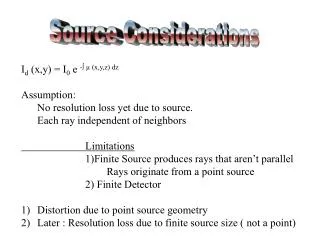
Source Considerations Id (x,y) = I0 e -∫ µ (x,y,z) dz Assumption: No resolution loss yet due to source. Each ray independent of neighbors Limitations 1)Finite Source produces rays that aren’t parallel Rays originate from a point source 2) Finite Detector Distortion due to point source geometry Later : Resolution loss due to finite source size ( not a point)
dr • (xd,yd) X-ray Source (x,y,z) d Id (xd,yd) = Ii (xd,yd) exp [ -∫µ0 (x,y,z) dr Photon density at Idetector First, what if no object?
Unit area on sphere is smaller than area it subtends on detector. So for unit area on detector, area on sphere reduces by cos(). Let N be the number of photons being emitted by the source. Unit area a Subtended area=acos() X-ray Source d Detector Plane For small solid angles Ω ≈ area/distance2 = a (cos )/r2 K energy per photon Divide by area a to normalize to detector area Obliquity Inverse Square Law
r d Normalize to Id (0,0) = I0 Now rewriting Ii in terms of I0 gives, But So, Ii= Io cos3 ()
r d Source Intensity ( Detector Coordinates) Id = Io cos3 cos() - Obliquity cos2 - Inverse Square Law
For a 40 cm FOV with x-ray source 1 m away, how much amplitude modulation will we have due to source obliquity?
Depth Dependent Magnification An incremental path of the x-ray, dr, can be described by its x, y, and z components. X-ray path is longer off axis
To study, let’s make intensity expression parametric in z. Each point in the body (x,y) can be defined in terms of the detector coordinates it will be imaged at. Then, rewriting an earlier description in terms of the detector plane. z/d describes minification to get from detector plane to object. Id (xd,yd) = Ii exp [ - ∫ µo ((xd/d)z, (yd/d)z, z) dz]
Putting it all together gives, Id = Io /(((1 + rd2)/d2)3/2) exp [ - ∫ µo ((xd/d)z, (yd/d)z, z) dz] source obliquity object obliquity
Two examples Object µ (x,y,z) = µo rect ((z - zo)/L) Object is not a function of x or y, just z. Id (xd,yd) = Ii exp [ - µo L]
Id (xd,yd) = Ii exp [ - µo L] If we assume detector is entirely in the near axis, rd2 << d2 (paraxial approximation) Then, simplification results, Id = Io e -µ0L
x out of plane Infinite in x Example 2 For µo (x,y,z) = µoP (y/L) P((z - z0)/w) Find the intensity on the detector plane Three cases: 1. Blue Line: X-Ray goes through entire object 2. Red Line: X-ray misses object completely 3. Orange Line: X-ray partially goes through object Id (xd,yd) = Ii exp [ - ∫ µo ((xd/d)z, (yd/d)z, z) dz]
Example 2 Id (xd,yd) = Ii exp [ - ∫ µo ((xd/d)z, (yd/d)z, z) dz] For the blue line, we don’t have to worry that the path length through the object will increase as rd increases. That is taken care of by the obliquity term For the red path, Id (xd,yd) = Ii For the orange path, the obliquity term will still help describe the lengthened path. But we need to know the limits in z to integrate
µo (x,y,z) = µoP (y/L) P((z - z0)/w) Example 2 If we think of thin planes along z, each plane will form a rect in yd of width dL/z. Instead of seeing this as a P in y, let’s mathematically consider it as a P in z that varies in width according to the detector coordinate yd. Then we have integration only in the variable z. The P define limits of integration
P in y dimension P in z dimension z z0 z0 + w/2 z0 - w/2 -dL/2|yd| dL/2|yd| X-ray misses object completely As yd grows,first P contracts and no overlap exists between the P , functions. No overlap case when dL/2yd <z0 – w/2 |yd | > dL/(2 zo -w ) Id = Ii
P in y dimension P in z dimension z z0 z0 + w/2 z0 - w/2 -dL/2|yd| dL/2|yd| X-ray goes completely through object As yd 0, x-ray goes completely through object This is true for dL/2yd >z0 + w/2 |yd |< dL/ (2 zo + w) Id = Ii exp {-µo w}
P in y dimension P in z dimension z z0 z0 + w/2 z0 - w/2 -dL/2|yd| dL/2|yd| • Partial overlap case. Picture above gives the limits of integration. min { zo + w/2 dL/2|yd| Id = Ii exp {-µo ∫ - dz} • min {zo-w/2 • dL/2|yd|
3) Id = Ii exp {-µo ((dL/ 2|yd | ) + w/2 - zo)} X-rays miss object X-rays partially travel through object X-rays go entirely through object The above diagram ignores effects of source obliquity and the factor in the exponential How would curve look differently if we accounted for both of these?
Thin section Analysis See object as an array of planes µ (x,y,z) = (x,y) (z - z0) Analysis simplifies since only one z plane where M = d/z0 represents object magnification If we ignore obliquity, Or in terms of the notation for transmission, t, Note: No resolution loss yet. Point remains a point.
Finite Source Instead of a point source, let’s consider a more realistic finite source. The source will be planar and parallel to the detector. We will consider it as an array of point sources. Here we will consider half a doughnut as an example, s(xs,ys). ys xd xs yd Image of Source s(xs,ys) d-z Find the result in the detector plane as a result of the sum of source points z d
Geometric Ray Optics Low m Response to pinhole impulse at origin Planar Object In the Fourier domain, Id (u,v) = KM2m2 T (Mu, Mv) S (mu,mv)
small m Large m u z < d Geometric Ray Optics Low m In the Fourier domain, Id (u,v) = KM2m2 T (Mu, Mv) S (mu,mv) Object is magnified by Source causes distortion Id (u,v) Curves show S(mu,mv) for a large m and a small m