Download
1 / 72
830 likes | 1.27k Vues
Very High Radix Montgomery Multiplication. David Harris, Kyle Kelley and Ted Jiang Harvey Mudd College Claremont, CA Supported by Intel Circuit Research Labs. Outline. RSA Encryption Montgomery Multiplication Radix 2 Implementations Tenca-Koç Radix 2 Improved Radix 2

E N D
Very High Radix Montgomery Multiplication David Harris, Kyle Kelley and Ted Jiang Harvey Mudd College Claremont, CA Supported by Intel Circuit Research Labs
Outline • RSA Encryption • Montgomery Multiplication • Radix 2 Implementations • Tenca-Koç Radix 2 • Improved Radix 2 • Very High Radix Implementations • Very High Radix • Parallel Very High Radix • Quotient Pipelining • Results • Future Work
RSA Encryption • Most widely used public key system. • Good for encryption and signatures. • Invented by Rivest, Shamir, Adleman (1978) • Public e and private d keys are long #s • n = 256-2048+ bits • Satisfy xde mod M = x for all x • Finding d from e is as hard as factoring M • Encryption: B = Ae mod M • Decryption: C = Bd mod M = Aed = A
RSA Derivation • Choose two large random primes p, q • M = pq • Totient: f = (p-1)(q-1) • Public key e • e is coprime to f • Private key d • such that de = 1 mod f • Then xed mod M = x • According to Fermat’s Little Theorem
Cryptographic Algorithms • DES, AES • Symmetric key algorithms • Require exchange of secret key • Computationally efficient • RSA, ECC • Public key algorithms • No key exchange needed (e.g. ecommerce) • Computationally expensive • Use public key to exchange symmetric key
Modular Exponentiation • Critical operation in RSA and for • Digital signature algorithm • Diffie-Hellman key exchange • SSL, IPSec, IPv6 • Elliptic curve cryptosystems • Done with modular multiplications • Ex: A27 = ((((((A2) * A)2)2) * A)2) * A • Division after each multiplication to compute modulo • Maximum 2n, average 1.5n mults needed
Binary Extension Fields • Building blocks are polynomials in x • Operations performed modulo some irreducible polynomial f(x) of degree n • Arithmetic done modulo 2 • Called GF(2n) • Example: GF(23) • 0, 1, x, x+1, x2, x2+1, x2+x, x2+x+1 • Computation is the same as GF(p) • Except that no carries are propagated
Montgomery Multiplication • Faster way to do modular exponentation • Operate on Montgomery residues • Division becomes a simple shift • Requires conversion to and from residues only once per exponentiation
Montgomery Residues • Let the modulus M be an odd n-bit integer • 2n-1 < M < 2n • Define R = 2n • Define the M-residue of an integer A < M as • A = AR mod M • There is a one-to-one correspondence between integers and M-residues for 0 < A < M-1
Montgomery Multiplicaton • Define Z = MM(X, Y) = XYR-1 mod M • Where R-1 is the inverse of R mod M: R-1R = 1 (mod M) • Montgomery Mult finds residue of Z = XY mod M Z = X Y R-1mod M = (XR) (YR) R-1mod M = XYR mod M = ZR mod M
Montgomery Reduction Precompute M’satisfying RR-1 – MM’ = 1 Convert mult and mod to 3 mult and shift Multiply: Z = X × Y Reduce: reduce = Z × M’ mod R Z = [Z + reduce × M] / R Normalize: if Z ≥ M then Z = Z – M Why is Z + Reduce × M divisible by R? Mult Drop bits Mult Mult Shift for R-1
Reduction Proof [ Z + reduce × M ]mod R = [ Z + (Z × M’ mod R)× M ]mod R = [ Z + Z × M’M ]mod R = [ Z + Z(RR-1- 1)]mod R = ZRR-1mod R = 0mod R So Z + reduce × M is divisible by R
More Comments on M’ • RR-1 – MM’ = 1 • Implies M’ -M-1 mod R • M’ is odd • M’ is precomputed from M using the extended Euclidian algorithm • M is held constant over many mults • Only least significant v bits of M’ are needed when computing in radix 2v • Dusse & Kaliski, Eurocrypt ’90s
CPU Crypto Accelerators • VIA Esther Padlock Hardware Security • Montgomery Multiplier < 0.5 mm2 die area • Accessed by x86 instruction • 256b - 32Kb keys in 128 bit granularity • Also supports AES • SmartMIPS Smart Card Extensions • RSA, ECC, AES applications • GF(2n) multiply, MAC instructions • Carry propagation for multiword adds • AES permutations and rotations • Intel LaGrande Technology • Trusted computing
Embedded Crypto Accelerators 3COM Router 5000 Series Encryption Accelerator IBM PCI SSL Cryptography Accelerator
Radix 2 Algorithm • In radix 2, process one bit of X per step • Reduction becomes trivial because M’ mod 2 = 1 • Two multiplies and one shift per step Z = 0 for i = 0 to n-1 Z = Z + Xi × Y reduce = Z0 trivial Z = Z + reduce × M make Z divisible by 2 Z = Z/2 if Z ≥ M then Z = Z – M final Mod M Z = X × Y reduce = Z × M’ mod R Z = [Z + reduce × M] / R if Z ≥ M then Z = Z – M
Final Modulo • Result before last step in range • 0 Z < 2M • Reducing Z-M at the end is a hassle • Allow 0 X, Y < 2M to avoid reduction • Then if R > 4M, 0 Z < 2M • Hence add two bits to R to avoid subtraction at end of each step Walter, Electronic Letters ’99
Conversion • Conversion of integers to/from Montgomery residues takes one MM operation (if r2 mod M is precomputed and saved): • Modular exponentiation takes two conversion steps and ~2n multiplication steps.
Reconfigurable Hardware • Building hardwired n-bit unit is limiting • Slow for large n • Not scalable to different n • Better to design for w-bit words • Break n-bit operand into e w-bit words • e = n/w • This is called scalable • Also handle both GF(p) and GF(2n) • Requires conditionally killing carries • Called unified
Tenca-Koç Montgomery Multiplier M = (M(e-1), …, M1, M0), Y = (Y(e-1), …, Y1, Y0), Z = (Z(e-1), …, Z1, Z0), X = (Xn-1, …, X1, X0) Z = 0 for i = 0 to n-1 (Ca, Z0) = Z0 + Xi × Y0 reduce = Z0 (Cb, Z0) = Z0 + reduce × M0 for j = 1 to e (Ca,Zj) = Zj + Ca + Xi × Yj (Cb,Zj) = Zj + Cb + reduce × Mj Zj-1 = (Zj0, Zj-1w-1:1) Tenca, Koç, Trans. Computers, 2003
Processing Elements • Keep Z in carry-save redundant form • Tc = 2tAND + 2tCSA + tMUX + tBUF(w) + tREG
Parallelism • Two dimensions of parallelism: • Width of processing element w • Number of pipelined PEs p • Multiply takes k = n/pkernel cycles
Queue • If full PEs cause stall, queue results • Convert back to nonredundant form • Saves queue space • CPA needed for final result anyway
Improved Design • Don’t wait two cycles for MSB • Kick off dependent operation right away on the available bits • Take extra cycle(s) at the end to handle the extra bits • For p processing elements, cycle count reduces from 2p to p + (p/w) Harris, Krishnamurthy, Anders, Mathew, Hsu, Arith 2005.
Improved PE • Left-shift M and Y • Rather than right-shift Z • Same amount of hardware
Latency • Tenca-Koç k(e+1) + 2(p-1) n > 2pw – w k(2p+1) + e - 2 n 2pw – w • Improved Design (k+1)(e+1) + p-2 n > pw k(p+1) + 2e - 1 n pw
Very High Radix • Handle many bits of X at a time • Radix 2v processes v bits of X • Only f = n/v outer loop iterations needed • k = n/pv kernel cycles with p PEs • Hardware changes • w bit AND vw bit multiplier • Right shift by v bits after each step • Use vw so bits are available to shift • Cycle time gets longer • Reduce becomes more complicated • Must drive v lsbs to 0
Very High Radix Algorithm Z = 0 for i = 0 to f-1 Z = Z + Xi× Y reduce = (M’ × Z) mod 2vreduce bottom v bits Z = Z + reduce× M Z = Z / 2v Z = X × Y reduce = Z × M’ mod R Z = [Z + reduce × M] / R
Scalable Very High Radix MM Z = 0 for i = 0 to f-1 (CA, Z0) = Z0 + X0× Y0 reduce = (M’ × Z0) mod 2vonly reduce bottom v bits (CB, Z0) = Z0 + reduce× M0 for j = 1 to e + (v + 1) / w - 1 (CA, Zj) = Zj + CA + Xi × Yj (CB, Zj) = Zj + CB + reduce× Mj Zj-1 = (Zjv-1:0, Zj-1w-1:v) 2 mul, 1 shift in inner loop
Very High Radix PE Kelley, Harris IWSOC 2005
Pipeline Timing Each MAC is given a full cycle Tc = tMUL(v,w) + tCPA(v+w) + tmux + tREG Two MAC columns for each PE Four cycle latency between PEs: 1) Z0 = Xi × Y0 2) reduce = M’ × Z0 mod 2v 3) Z0 = Z0 + reduce × M0 4) Z1 = Z1 + reduce × M1, shift into Z0
Very High Radix Latency k(e + 3) + 4(p - 1) + 2 n > 4pw – 2w k(4p + 1) + (e - 1) n 4pw – 2w • Design limited for small n by 4-cycle latency between PEs
Parallel Very High Radix • Eliminate two of the cycles • Multiplication to compute reduce • By precomputing M = M’ × M mod R • Dependency of Z0 on reduce • By prescaling X by 2v so Z0 = 0 • Math proposed by Orup Arith95 • But no scalable very high radix HW ~
Improvement 1: Eliminate Multiply Z = X × Y reduce = Z × M’ mod R Z = [Z + reduce × M] / R Z = 0 for i = 0 to f-1 Z = Z + Xi× Y Z = Z + Z0× M M = (M’ mod 2v)M mod R Z = Z / 2v ~ M = M’ × M mod R (precompute) Z = X × Y Z = [Z + Z × M] / R ~ ~ ~
Improvement 2: Prescale X by 2v Z = 0 for i = 0 to f-1 Z = Z + Xi× Y Z = Z + Z0× M Z = Z / 2v One more iteration Z = 0 for i = 0 to f Z = Z + 2vXi× Y + Z0× M Z = Z / 2v Z = 0 for i = 0 to f Z = (Z + Z0× M) / 2v + Xi× Y ~ ~ Because Z0 is independent of 2vXi ~ Final result in range 0 Z < 2n+v+1 - avoid final small mod in successive mults by using larger R
Improvement 3: Avoid LSW add Z = 0 for i = 0 to f Z = (Z + Z0× M) / 2v + Xi× Y Z = 0 for i = 0 to f reduce = Z0 Z = Z >> v + reduce × M+ Xi× Y ~ ~ (Z + Z0× M) /2v = Z >> v + (Z0 × M + Z mod2v) /2v = Z >> v + (Z0× (M+1)) / 2v = Z >> v + Z0× M ~ ~ ~ M + 1 M = 2v ~ M M’M -1 mod 2v So M + 1 is divisible ~
Scalable Parallel Very High Radix Z = 0 for i = 0 to f C = 0 reduce = Z0 for j = 0 to e + v/w (C, Zj) = Zj+ C + reduce× Mj+Xi× Yj Zj-1 = (Zjv-1:0, Zj-1w-1:v)
Parallel Very High Radix PE Kelley, Harris Asilomar 2005
Pipeline Timing Tc = tMUL(v,w) + 2tCSA + tCPA(v+w) + tREG Two cycle latency between PEs: 1) Z0 = Z0 + Xi × Y0 + reduce × M0 2) Z1 = Z1 + Xi × Y1 + reduce × M1, shift into Z0
Parallel Very High Radix Latency k(e+1) + e+1 + 2(f mod p) n > 2pw – v k(2p+1) + e+1 + 2(f mod p) n 2pw – v
Quotient Pipelining • Reduce depends on previous Z • Pipeline reduce calculation to avoid reduce being on the critical path • Parallel Very High Radix can be viewed as 0-stage Quotient Pipeline architecture
0-stage Quotient Pipelining • Parallel Very High Radix • reduce× Mjand Xi× Yj occurs simultaneously • Require reduce in non-redundant form • Solution: Delay reduce× Mjcalculation by d PE’s: d-stage delay Quotient Pipelining
d-Stage Delay Quotient Pipelining • Parallel Design • M = (M’ mod 2v) × M >> v • reduce produced by PEi is used by PEi+1 • Quotient Pipelining • M = (M’ mod 2v(d+1)) × M >> v(d+1) • Where d is the # of delay stages • Reduce produced by PEi is used by PEi+1+d • Parallel: d = 0-Stage Quotient Pipelining
1-Stage Quotient Pipelined Algorithm Z = 0 oldreduce = 0 for i = 0 to f reduce = Z0 Z = Z >> v + oldreduce × M+ Xi× Y oldreduce = reduce Z = Z << v + oldreduce
1-Stage Scalable Quotient Pipelining Z = 0 oldreduce = 0 for i = 0to f C = 0 reduce = Z0 for j = 0 to e (C, Zj) = (Zjv-1:0, Zj-1w- 1:v) + oldreduce × Mj +Xj × Yj + C oldreduce = reduce Z = Z << v + oldreduce