Some Background
This article discusses the need for better utilization of wind data in weather and climate analyses. It highlights the limitations of current models and the potential of satellite data for measuring winds in the planetary boundary layer (PBL). The article also explores the importance of accurate wind measurements for improving storm definition and climate models.

Some Background
E N D
Presentation Transcript
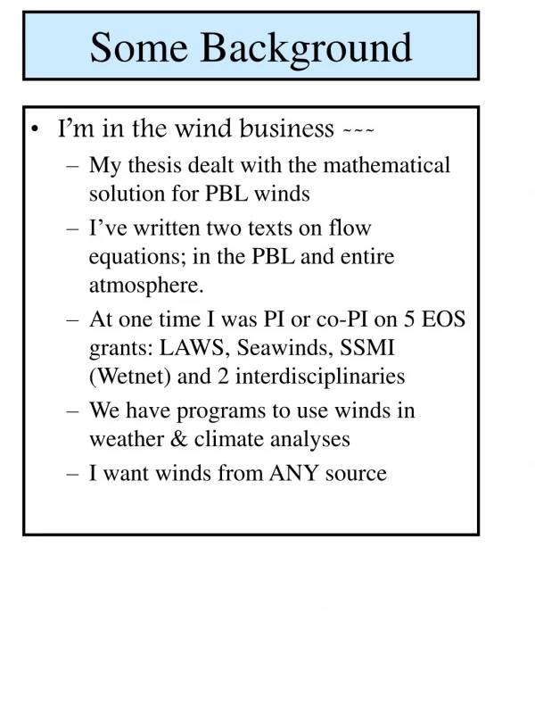
Some Background • I’m in the wind business --- • My thesis dealt with the mathematical solution for PBL winds • I’ve written two texts on flow equations; in the PBL and entire atmosphere. • At one time I was PI or co-PI on 5 EOS grants: LAWS, Seawinds, SSMI (Wetnet) and 2 interdisciplinaries • We have programs to use winds in weather & climate analyses • I want winds from ANY source
Winds are not --- have never been --- on NASA/s menu. Why? • I surveyed EOS investigators: “It is assumed that the winds will be provided by GCMs” • Scatterometer data showed this is not true: • Missing storms, details • PBL Winds unphysical, often too low • Mainly a resolution problem, but also because GCMs cannot handle Turbulence in many cases (PBL, Conv. Towers, tropopause, jets….) or sub-grid organized flow (OLE).
The Need for Winds
Applications Better GCM Progs Better Storms Definition Higher Winds (heat fluxes) Better Climate Models Little Science things like: Proof of ubiquity of Rolls (OLE) RABrown 2001
A Winds Motivation • High Marine Surface Winds do not appear in: • Buoy data • Climate records • General Circulation Models • Satellite sensor algorithms • High Marine Surface Winds do appear in: • Ocean Meteorology Ship reports • Dedicated Airplane PBL Flights • A PBL model that includes OLE • Higher winds imply higher heat fluxes in climatology; revised ocean mixed layer models. R.A. Brown, 1997, 2000; ‘01
There exists an opportunity for satellite data • Measurements from sondes, ships & buoys incur large errors due to turbulence & OLE • There are few measurements of winds in the PBL in situ • There are no satellite determined winds IN the PBL • The fluxes (air-surface) require boundary layer winds • Climate Analyses have been made on extremely poor climatology data R. A. Brown 1/2001
The Available Winds (1990-2005)
Sources of Surface Wind Fields for Climate Studies • From Surface Measurements • Ships & Buoys • Radiosondes • From Models • GCM (with K-theory PBLs) • UW Similarity Model (with OLE) R.A. Brown, 1997, 2001
Satellite Wind Sensors • Scatterometers ERS (ESA); Quikscat (USA) (2001 - ); SeaWinds on Adeos (USA,Japan) (2002); AScat (ESA) (2004) • SARs ERS (ESA); Radarsat (Canada); Envisat (ESA) ********** • Passive Radiometers Windsat (USA) (2002) • Lidars ESA (2008)
Scatterometer wind fields here Pressure field SAR Wind field
Theory A conversation in 1977: Businger to Brown: “You’re a fluiddynamacist, we’d like the solution to the relation between the surface wind and the wave generation” Brown to Businger: “OK” (I know it’s impossible, but it’s a living) Bottom line: (20 years later) There is no proven theory for wind generation of waves. However, in the best tradition of Atmospheric Science --- there is a curve fit Epilogue: Satellite Data Prove PBL Winds Theory
Appraisal of Basics: Theory for Scatterometer, SAR, radiometer Data: cm-scale, average density of capillaries and short gravity waves in a footprint. 50km 25km 7km 100m (SAR) • Theory: State: 1-10, poor to excellent • Wind generation of water waves 1 • % energy into short/long waves 2 • Wave-wave interaction 3 • Surface layer wind 8 • PBL wind (without OLE) 4 (with OLE) 8 R.A. Brown 2001
Appraisal of Basics: Microwave Data from Scatterometry, SAR, Radiometers Data: cm-scale, average density of capillaries and short gravity waves in a footprint. 50km 25km 7km 100m (SAR) And surface ‘truth’ wind. Parameterizations State: 1-10, poor to excellent U10 (u*) land 8 U10 (u*) ocean 5 PBL U(z) (similarity) 7 Scatterometer Model Function u* (o) 4 U10 (o) 8 P (o) 7 R.A. Brown 2001
Practical Aspects of Wind Measurements (Surface ‘Truth’ Limits) Ship winds: Sparse and inaccurate (except Met. Ships). Buoy winds: Sparse; a point. Tilt; variable height - miss high winds and low wind directions. GCM winds: Bad physics in PBL Models; Toolow high winds, too high low winds. Resolution coarse (getting better). Satellite winds: Lack good calibration data. Resolution (”). 11-99, 5/00, 7/01 RAB
Height meters The Surface Layer = the log layer = the law of the wall 200 U10/VG 0.7 100 V
Practical Aspects of a Geostrophic Wind Model Function (Pressures) • Surface ‘Truth’ Limits • Radiosondes (winds) • Sparse; NG in PBL • Buoy and ship pressures:Accurate in low and high wind regimes; sparse • GCM (winds & pressures): • Poor winds. Good pressure verification, compatible 11-99, 7/01 RAB
Geostrophic Flow 1-3 km VG(u*) effects Ekman Layer with OLE Thermal Wind Nonlinear OLE Gradient Wind Advection,centrifugal terms Non steady-state 0 – 100 m U10(u*) effects Stratification U10 Surface Layer Surface Stress, u* Variable Surface Roughness Ocean surface R.A. Brown PORSEC 2000
CONCLUSIONS • The surface layer relation, hence U10 {u*(o ) }works well 0 < z < 100 meters • There is almost no surface truth --- buoy or GCM surface winds with U10 > 25 m/s • The U10 model function can be extrapolated to about 35 m/s • There are indications that o responds to the sea state for U10>40 m/s. (H-pol > 60 m/s?) • There is a Model function yielding winds possibly to 60 m/s (2000) • The PBL model yields U(z), 0 < Z < 1 km (gradient) • Requires U10. • Requires Stratification Information RABrown, ’99; ‘01
The Struggle to get Satellite Wind Sensors
A Brief History of Scatterometers 1970 1980 1990 2000 2010 Conception SeaSat Built --- with Scat, SAR, SMMR, Alt SeaSat Launch --- Lasts 99 days NSCAT conceived and built Dark Ages: launch $ to gulf & carribean wars, refurbish battleships, 200 ship fleet, Star Wars ERS-1 Launch (turned off) NSCAT launched on ADEOS --- 9 mos. ERS-2 Launch Quikscat Launch Dark Ages 11 in USAI Star Wars 11 SeaWinds on ADEOS - II ESA A-SCAT R. A. Brown 1/2001
Programs and Fields available onhttp://pbl.atmos.washington.eduQuestionsto rabrown, neal or jerome@atmos.washington.edu • Direct PBL model: PBL_LIB. (’75 -’01) An analytic solution for the PBL flow with rolls, U(z) = f( P, To , Ta , ) • The Inverse PBL model: Takes U10 field and calculates surface pressure field (VG) P (U10 , To , Ta , ) (1986 - 2001) • Pressure fields directly from the PMF: P (o) along all swaths (exclude 0 - 5° lat) (2001; in progress) • Surface stress fields from PBL_LIB corrected for stratification effects along all swaths (2001; in progress) R.A. Brown 2000, ‘01