AMDAR (aircraft) and Radar Data Assimilation
450 likes | 675 Vues
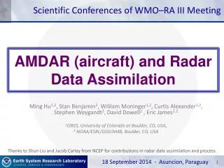
Scientific Conferences of WMO –RA III Meeting. AMDAR (aircraft) and Radar Data Assimilation. Ming Hu 1,2 , Stan Benjamin 2 , William Moninger 1,2 , Curtis Alexander 1,2 , Stephen Weygandt 2 , David Dowell 2 , Eric James 1,2 1 CIRES , University of Colorado at Boulder, CO, USA,

AMDAR (aircraft) and Radar Data Assimilation
E N D
Presentation Transcript
Scientific Conferences of WMO–RA III Meeting AMDAR (aircraft) and Radar Data Assimilation Ming Hu1,2, Stan Benjamin2, William Moninger1,2, Curtis Alexander1,2, Stephen Weygandt2, David Dowell2 , Eric James1,2 1CIRES, University of Colorado at Boulder, CO, USA, 2 NOAA/ESRL/GSD/AMB, Boulder, CO, USA Thanks to Shun Liu and Jacob Carleyfrom NCEP for contributions in radar data assimilation and process 18 September 2014 - Asuncion, Paraguay
What is Data Assimilation • Numerical Weather Prediction (NWP) is an initial-condition problem • Given an estimate of the present state of the atmosphere (initial conditions), and appropriate surface and lateral boundary conditions, the model simulates (forecasts) the atmospheric evolution • The more accurate the estimate of the initial conditions, the better the quality of the forecasts (“accurate” doesn’t mean to fit to the observations very close) • Data Assimilation: The process of combining observations and short-range forecasts to obtain an initial condition for NWP • The purpose of data assimilation is to determine as accuratelyas possible the state of the atmospheric flow by using all available information for NWP
Data Assimilation: Variational Method (VAR) • Jis called the cost function of the analysis (penalty function) • Jb is the background term • Jois the observation term • The dimension of the model state is n and the dimension of the observation vector is p: • xt true model state (dimension n) • xb background model state (dimension n) • xa analysis model state (dimension n) • yvector of observations (dimension p) • H observation operator (from dimension n to p) • B covariance matrix of the background errors (xb – xt) (dimension nn) • R covariance matrix of observation errors (y – H[xt]) (dimension pp) J(x) = (x-xb)TB-1(x-xb)+(y-H[x])TR-1(y-H[x]) = Jb + Jo In this talk, we will use variational method to explain AMDAR and Radar data assimilation but most of steps are same for Ensemble based data analysis method
VAR: Background Term • Background (forecast field): xb • Analysis: x • Start from x=xb • Analysis increment: x-xb • Background error covariance: B • Variance: the background quality • Correlation • Horizontal and vertical relation between 2 analysis point • Balance: relation between two analysis variables J(x) = (x-xb)TB-1(x-xb)+(y-H[x])TR-1(y-H[x])
VAR: Observation Term • Observation: y • Observation operator: H[x] • Conventional observation: • T, wind, moisture, Ps • 3D interpolation • Non-conventional observations: • Radiance, Radar, GPSRO, … • Complex function • Observation innovation: y-H[x] • Observation error variance: R • Assumption: No correlation between two observations J(x) = (x-xb)TB-1(x-xb)+(y-H[x])TR-1(y-H[x]) x x x x x x x x y x x x x y x x x x
VAR: Steps of using observations Step 1: Understand observations Y • Name • Variables observed • Geographic and time distribution • Space and time resolution • Observation errors • Quality Control and bias correction • Acceptable format (BUFR,…) • … J(x) = (x-xb)TB-1(x-xb)+(y-H[x])TR-1(y-H[x]) 1 2 3 1 2 Background term are the same for all observations Step 2: Build observation operator: link analysis variables x to observations H[x] • Conventional observations: • AMDAR observations • 3D interpolation • Non conventional observations: Complex function • Radar Reflectivity = f(qr, qs, qh) • Radar radial wind=f(u, v, w) Step 3: Define observation error variance R
AMDAR data assimilation • Understand AMDAR (commercial aircraft) Data • What is AMDAR • What is observed • Data coverage and resolution • Observation errors • Quality control and bias correction • Use AMDAR data in data assimilation • The impact of the AMDAR data • Regional NWP system (Rapid Refresh for US/NCEP) • Global NWP system (ECMWF)
Understand AMDAR Data • AMDAR: Aircraft Meteorological Data Relay • AMDAR is the automated measurement and transmission of meteorological data from an aircraft platform • The AMDAR observing system is now recognized by WMO as a critical component of the WMO Global Observing System(GOS)
What is observed in AMDAR • Vertical profiles are derived as the aircraft is on ascent or descent • en-routed dataare derived at cruise altitudes of around 35,000 feet (10,500 meters). • The meteorologicalparameters can be measured or derived: • Air temperature (static air temperature) • Wind speed and direction • Pressure altitude (barometric pressure) • Turbulence (Eddy Dissipation Rate or Derived Equivalent Vertical Gust) • Additional non-meteorological parametersinclude: • Latitude position • Longitude • Time • Icing indication (accreting or not accreting) • Departure and destination airport • Aircraft roll angle • Flight number • A water vapor (humidity) measurement can also be derived • Water vapor sensor: The Water Vapor Sensing System 2nd Generation (WVSS-II) • Operationally in the USAand Europe Temperature , Wind, Pressure Location, time, flight number Humidity
List of AMDAR Participating Airlines • As of July 2013, more than 400,000 observations per day world wide • 2863 aircraft are currently reporting world-wide, not including Aeromexico data (coming soon) since 1-Aug-2014
24h AMDAR Data Coverage Typically, every 5-10 minutes of regular real-time reports of meteorological variables whilst en-route at cruise level
AMDAR Vertical profiles Denver Descent Sounding LAS Vegas Ascent Sounding • High resolution vertical profiles: • High-reso profiles are reported every 300 feet in low level and every 1000 feet in middle and upper • Number vary a lot by airport: • Busy airport during the day : every 15 min or less • Many: couple profiles per day • Details in http://amdar.noaa.gov/new_soundings/2014_08_31.html Montreal Ascent Sounding (No moisture)
Time in plots is US mountain time. AMDAR data coverage over US 00 – 03 night 03 – 06 early morning 06 – 09 morning Obs Number Big various during day and night 09 – 12 day 12 – 15 day 21 – 00 early night 18 – 21 afternoon 15 – 18 day
AMDAR data coverage over S. America 05-08 23-02 02-05 17-20 20-23 night Early morning Late afternoon to early night Time in plots is local time in Asuncion, Paraguay Most of observations are during the night time 14-17 08-11 11-14 During the day time
Data Quality • The expected uncertainties for basic AMDAR data parameters (based on AMDAR Reference Manual): • Data analysis uses tunedobservation errors AMDAR observation error used by GSI for US NAM and RAP applications
AMDAR data quality control • GSD AMDAR Rejectionlist: • Week-long statistics • Used by us to generate daily aircraft reject lists for RAP and 3km HRRR (GSD/NOAA regional models) • Used actively by NWS and other centers • Statistics of aircraft obs against Rapid Refresh 1-h forecasts: • bias_T> 2 (°C), std_T> 2 (°C), • bias_S> 2 (m/s), std_S> 5 (m/s), • bias_DIR> 7°, std_DIR> 30°, • std_W> 5(m/s), rms_W> 7(m/s), • bias_RH> 10%, std_RH> 20%, Example of GSD AMDAR rejection list: ;tailerrors FSL MDCRS N bs_TStd_Tbs_Sstd_Sbs_Dstd_Dstd_Wrms_Wbs_RHstd_RH (failures) 00000400 T W R 0 -------- 0 0.0 0.0 0.0 0.0 0 0 0.0 0.0 0.0 0.0 UND_Piper ( resrch_T_W_R ) 00000450 T W R 0 -------- 0 0.0 0.0 0.0 0.0 0 0 0.0 0.0 0.0 0.0 UND_Piper ( resrch_T_W_R ) EU8001 - W - 10081 10081 409 -0.5 0.9 0.5 6.1 -1 15 7.4 9.1 0.0 0.0 Unknown ( std_Sstd_Wrms_W ) N194AA - W - 2777 2777 483 0.2 0.7 0.4 1.6 -7 14 1.2 2.3 0.0 0.0 Unknown ( bias_DIR ) N203WN T - - 11060 11060 3085 2.6 1.2 0.2 2.4 1 8 1.8 3.5 -7.6 13.5 Unknown ( bias_T ) N220WN T - - 11002 11002 3268 2.7 1.3 0.3 2.2 1 11 1.8 3.4 -9.2 16.7 Unknown ( bias_T ) N402WN - - R 11149 11149 2853 -0.3 0.8 0.1 2.3 1 10 1.8 3.4 6.5 29.1 Unknown ( std_RH ) N407WN - - R 11087 11087 2459 -0.4 1.3 1.0 2.6 -1 10 2.2 4.0 0.4 21.6 Unknown ( std_RH ) N421LV T - - 10973 10973 2948 3.5 1.2 0.3 2.0 -1 7 1.4 2.9 0.0 0.0 Unknown ( bias_T ) Which observed variables to reject Aircraft tail number
GSD Aircraft Rejection List Vector wind difference between AMDAR observations and RR 1h forecasts. Shows some obvious bad aircraft winds near Chicago. (Used by NWS to help identify bad aircraft data.)
Bias of AMDAR obs and bias correction • Comparing with RAOBs, AMDAR temperature observations are biased: • At flight levels, AMDAR have a warm bias. (BUT RAOBs have a cold bias at the same level (ref 1). So exactly how to balance these two biases to move the model temperature toward the truth is a difficult --and somewhat philosophical--question) • Bias can be dependent to fly phase (ref 2): • Descent: a strong cool bias • Ascent: a slight warm bias • Bias correction (BC) to the AMDAR observations • ECMWF: variational aircraft temperature BC • NCEP: testing similar method as ECMWF with GSI • NASA/GMAO: bias calculated after analysis and var method BominSun, Anthony Reale, Steven Schroeder, Dian J. Seidel and Bradley Ballish (2013) Toward improved corrections for radiation-induced biases in radiosonde temperature observations. JGR 118, 4231-4243. Barry Schwartz and Stanley G. Benjamin, 1995: A Comparison of Temperature and Wind Measurements from ACARS- Equipped Aircraft and Rawinsondes. Wea. Forecasting, 10, 528–544.
Use AMDAR data in analysis • Observation operator for AMDAR data: • Conventional observations: T, Q, U, V • 3D interpolation from grid analysis field to observation location • Same as other conventional observation, such as sounding and surface observations • Better to define a data type for AMDAR, for example, in NCEP PrepBUFR:
Use AMDAR data in analysis • Convert data to the values and format analysis system accepts. Use GSI as an example: • Convert AMDAR data into temperature, U and V component of wind observation, specific humidity • Encode the observations into PrepBUFR file with all other conventional observations. • Let analysis system run … • After analysis, must check the analysis impact: • How many observations are used in the analysis • The distribution of the analysis increment over analysis domain in one analysis • Data impact from OSE, …
AMDAR data impact: RAP • The Rapid Refresh (RAP) is a US operational hourly updated regional numerical weather prediction system for aviation and severe weather forecasting. • Configuration: • 13 km horizontal North American grid • Twice daily partialcycles from GFS atmospheric fields • Hourly continuecycledland-surface fields • Model: • WRF-ARW dynamic core • Data Assimilation: • GSI 3D-VAR/GFS-ensemble hybrid data assimilation • GSI non-variational cloud/precipitation hydrometeor (HM) analysis • DiabaticDigital Filter Initialization (DDFI) using hourly radar reflectivity observation RAP version 1 operational implementation: 01 May 2012 RAP version 2 operational implementation: 24 February 2014
Impact of AMDAR moisture in RAP Valid 00z - daytime RAP 2013 RH– national – 1000-400 hPa #1 obs type = aircraft Distant #2 tie – Surface, GPS, raobs Valid 12z - nighttime 12z and 00z combined
Impact of AMDAR Temp in RAP flight levels - 300-100 hPa national - 1000-100 hPa Valid 00z - daytime Valid 12z - nighttime 12z and 00z combined #1 = Aircraft #2 = RAOBs, surface Aircraft more impact at 3h, more at flight levels
Impact of AMDAR wind in RAP RAP Domain US CONUS region Valid 00z - daytime Valid 12z - nighttime 12z and 00z combined Wind - national – 300-100 #1 = Aircraft #2 = RAOBs, Some impact from sfc, GPS-Met, AMVs
AMDAR data impact (ECMWF) From The Benefits of AMDAR to Meteorology and Aviation (WIGOS Technical Report 2014-1, Version 1, Jan 2014) Available one line: https://docs.google.com/file/d/0BwdvoC9AeWjUbG1MRlAyU0dhZEk/edit
Radar data assimilation • Understand Radar Data • What is weather Radar • What is observed • Data coverage and resolution from single radar • Observation errors • Radar data Quality Control • Radar observation operator • Assimilate radar reflectivity data with DDFI and the data impact in RAP
What is weather radar • Weather radar, also called weather surveillance radar (WSR) and Doppler weather radar, is a type of radar used to locate precipitation, calculate its motion, and estimate it type (rain, snow, hail etc.) • Modern weather radars are mostly pulse-Doppler radar, capable of detecting the motion of rain droplets (radial velocity) in addition to the intensity of the precipitation (reflectivity) • Both types of the data can be analyzed to determine the structure of stormsand their potential to cause the severe weather
Radar Coordinate and Resolution Radar coordinate: The radar is located at the origin of the coordinate system; the Earth’s surface lies in the x-y plane: Azimuth angle Θ ; Elevation angle α; Range R. • WSR88D data resolution: • Beam width: 1 degree • Scan levels (tilt): 14 scans • Maximum range: 230 km • Gate resolution: • 250 m for Radial wind • 1 km for reflectivity • Products update every 6 minutes α
Understand 3D radar coverage The approximate height and width of the radar beam with distance from the radar site. Values in red represent the different elevation angles in this VCP 3 dimensional radar coverage from ground level Maury Markowitz - Own work
US Radar Coverage reflectivity • One of the only networks of fairly comprehensive, storm-scale data Radial velocity Courtesy of Jacob Carleyfrom NCEP
Radar Data Quality Control at NCEP • To meet the high standard required by data assimilation, it is necessary to develop simple and efficient QC technique for operational applications. • Radar data quality control is a necessary and initial step for operational applications of radar data. • Develop statistically reliable QC techniques for automated detection of QC problems in operational environments • Among various of radar data quality problems, radar measured velocities can be very different (≥10 m/s) from the air velocities in the presence of migrating birds. Courtesy of Shun Liu from NCEP
Radar data QC at NCEP Composite reflectivity Scatter plots of radial wind Before QC Before QC after QC after QC composite dual-pol variable CC Courtesy of Shun Liu; more details see Shun Liu’s talk at GSI tutorial 2010: http://www.dtcenter.org/com-GSI/users/docs/presentations_2010.php Or Shun Liu, et al: WRS-88D Radar Data Processing at NCEP. Submitted to Wea. Forecasting.
Radial Velocity Operator • No term for the vertical velocity (w) in GSI • Suggest only radial velocity observations from lower elevations should be considered • Avoid contamination of the horizontal wind field, especially due to hydrometeor sedimentation Vr(θ, α)=u cosαcosθ + v cosα sinθ +[w sinα] 90° - azimuth angle θ Elevation angle α Wind components from background Courtesy of Shun Liu and Jacob Carley from NCEP
Reflectivity Operator (example) From model forecast rain, snow, hail mixing ratio: qr, qh, qs hail rain snow T <= 0 °C (dry snow) T > 0 °C (wet snow) To David C. Dowell, Louis J. Wicker, and Chris Snyder, 2011: Ensemble Kalman Filter Assimilation of Radar Observations of the 8 May 2003 Oklahoma City Supercell: Influences of Reflectivity Observations on Storm-Scale Analyses. Mon. Wea. Rev., 139, 272–294.
Example of Radial Velocity Data analysis with GSI Full wind vectors Wind analysis Increment Radar reflectivity at 0900 UTC on 23 May 2005 Upper row: Analysis using default decorrelation length Low row: Analysis using a 1/4th of the default decorrelation length Need to modify Background Error Matrix to improve Rv Courtesy of Shun Liu from NCEP
Reflectivity data assimilation in RAP/HRRR Radar reflectivity data are assimilated through Diabatic digital filter initialization (DDFI) -20 min -10 min Initial +10 min + 20 min Backwards integration, no physics Forward integration,full physics with radar-based latent heating Initial fields with improved balance, storm-scale circulation RUC / RAP/ HRRR model forecast + RUC/RAP Convection suppression
Impact of DDFI with reflectivity Upper-level Divergence Low-level Convergence NSSL radar reflectivity (dBZ) K=17 U-comp. diff (radar - norad) K=4 U-comp. diff (radar - norad) 14z 22 Oct 2008 Z = 3 km
Radar Reflectivity Verification Eastern US, Reflectivity > 25 dBZ 11-21 August 2011 CSI 13 km CSI 40 km HRRR radar RAP radar HRRR radar RAP radar HRRR no radar RAP no radar HRRR no radar RAP no radar • 3km HRRR forecasts improve upon RAP 13km forecasts, especially at coarser scales much better upscaled skill • Radar DDFI adds skill at both 13km and 3km
HRRR Radar Reflectivity Assimilation 3 km HRRR Run 14z 13z 15z Digital Filter Digital Filter Digital Filter 2009-12 3-km Interp 3-km Interp 3-km Interp 15 hr fcst 15 hr fcst 15 hr fcst HRRR 2013 introduction of 3-km data assimilation (DA) On 10 April 2013 Latency reduced 45 min to 1-2 hrs Digital Filter 2013 1 hr pre-fcst Obs GSI 3D-VAR 3-km Interp HM Obs GSI HM Anx 15 hr fcst Refl Obs
HRRR 2013 Pre-forecast Hour • Temperature Tendency (i.e. Latent Heating) = f(Observed Reflectivity) • LH specified from reflectivity observations applied in four 15-min periods • NO digital filtering at 3-km • Reflectivity observations used to specify latent heating in previous 15-min period as follows: • Positive heating rate where obs reflectivity ≥ 35 dBZ over depth ≥ 200 mb (avoids bright banding) • Zero heating rate where obs reflectivity ≤ 0 dBZ • Model microphysics heating rate preserved elsewhere -45 -30 -15 0 LH = Latent Heating Rate (K/s) p = Pressure Lv = Latent heat of vaporization Lf = Latent heat of fusion Rd = Dry gas constant cp = Specific heat of dry air at constant p f[Ze] = Reflectivity factor converted to rain/snow condensate t = Time period of condensate formation (300s i.e. 5 min) -60 -45 -30 -15 0 Model Pre-Forecast Time (min)
HRRR 3-km Reflectivity Assimilation NO 3-km radar DA 3-km radar DA Radar Obs 05z 18 May 2013 0-hr fcst 0-hr fcst 05z + 45min 45 min fcst 45 min fcst
HRRR Retrospective Statistical Verification Statistical RetrospectiveComparison 30 May - 04 June 2012 (55 matched runs) 3-km grid ≥ 35 dBZ Eastern US With 3-km DA Without 3-km DA With 3-km DA Without 3-km DA Optimal Bias = 1.0 Improved 0-2 hr convection
Real-time HRRR case study Moore, OK 20 May 2013 20 – 21 UTC Tornadic Supercell HRRR 13 UTC run 8 hr forecast valid 21 UTC HRRR Composite Reflectivity Observed Reflectivity