Effective Constraint Handling in Evolutionary Algorithms

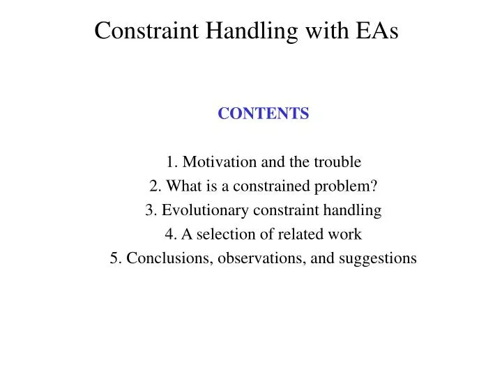
1. Constraint Handling with EAs CONTENTS 1. Motivation and the trouble 2. What is a constrained problem? 3. Evolutionary constraint handling 4. A selection of related work 5. Conclusions, observations, and suggestions

2. Motivation Why constraints? • Practical relevance: a great deal of practical problems are constrained. • Theoretical challenge: a great deal of untractable problems (NP-hard etc.) are constrained. Why evolutionary algorithms? • EAs show a good ratio of (implementation) effort/performance. • EAs are acknowledged as good solvers for tough problems.

3. The trouble with constraints and EAs Standard reproduction operators are blind to constraints. • Mutating a feasible individual can result in an infeasible new individual. • Recombining two feasible individuals can result in infeasible new individuals.

4. What is a constrained problem? Consider the Travelling Salesman Problem for n cities: • Let C = {city1, … , cityn} If we define the search space as • S = Cn, then we need a constraint requiring uniqueness of each city in an element of S • S = {permutations of C}, then we need no additional constraint. The notion ‘constrained problem’ depends on what we take as search space

5. What is constrained / free search? • Even in the space S = {permutations of C} we cannot perform free search • Free search: standard mutation and crossover preserve membership of S : mut()  S and cross(, t)  S • The notion ‘free search’ depends on what we take as standard mutation and crossover. • Standard mutation of x1, … , xn: • mut(x1, … , xn) =  x’1, … , x’n, x’i domain(i) • Standard crossover of x1, … , xn, y1, … , yn (and ...) • if for each child z1, … , zn: • zi {xi, yi} discrete case • zi [xi, yi] continuous case

6. Optimization Problems (FOPs) Free search space: S = D1 …  Dn • one assumption on Di: if it is continuous, it is convex • the restriction si Di is not a constraint, it is the definition of the domain of the i-th variable • membership of S is coordinate-wise, hence • a free search space allows free search Free Optimization Problem: S, f, • • S is a free search space • f is a (real valued) objective function on S • Solution of an FOP:  S such that f () is optimal in S FOPs are ‘easy’, in the sense that: • it's ‘only’ optimizing, no constraints and • EAs have a basic instinct for optimization

7. Constrained Optimization Problems (COPs) Constrained Optimization Problem: S, f, Φ • S is a free search space • f is a (real valued) objective function on S • Φ is a formula (Boolean function on S) Solution of a COP:  SΦ such that f() is optimal in SΦ • SΦ = { S | Φ() = true} is the feasible search space Φ is the feasibility condition – may be a combination of several constraints • In general with m constraints they will fall into two types: • inequalities: g_i(x) < 0 1…i…q • equalities h_i(x) = 0q+1 … i…m

8. S F X s n U Feasible & Unfeasible Regions • In general S will be split into two disjoint sets of spaces: • F (the feasible regions) • U (the unfeasible regions). • The spaces in F may be connected or not.

9. Constraint Satisfaction Problems (CSPs) Constraint Satisfaction Problem: S, •, Φ • S is a free search space • Φ is a formula (Boolean function on S) Solution of a CSP:  S such that Φ() = true Φ is typically given by a set (conjunction) of constraints ci = ci(xj1, … , xjni), where ni is the arity of ci ci Dj1 …  Djni is also a common notation FACTS: • the general CSP is NP-complete • every CSP is equivalent with a binary CSP (ni 2) Note that there is nothing to be optimized in a CSP

10. Examples • FOP: Schwefel function • S = D1 …  Dn Di = [-512.03, 511.97] • f() = 418.9829n - • COP: travelling salesman problem • S = Cn, C = {city1, … , cityn} • Φ() = true i, j  {1, … , n} i  j  si sj • f() = • CSP: graph 3-coloring problem • G = (N, E), E  N  N , |N| = n • S = Dn, D = {1, 2, 3} • Φ() = ΛeE ce(), where ce() = true iff e = (k, l) and sk sl

11. Solving CSPs by EAs (1) • EAs can only work if they have an f to optimize. Thus a CSP S, •, Φ must be transformed first to a Case 1. FOP: S, •, ΦS, f, • Case 2. COP: S, •, ΦS, f, Φ • The transformation must be (semi-)equivalent, i.e. at least the following implications must hold: 1. f () is optimal in S  Φ() 2. ψ () and f () is optimal in S  Φ() • Case 1: All constraints are handled indirectly, i.e. they are solved by `simply‘ optimizing in S, f, • e.g. f is number of violated constraints (to be minimized) • Case 2: Some constraints are handled indirectly (those transformed into f), some constraints are handled directly (those that remain constraints in ψ)

12. Solving CSPs by EAs (2) Constraint handling has two meanings: • 1. how to transform the constraints in Φ into f, respectively f, ψbefore applying an EA • 2. how to enforce the constraints in S, f, Φwhile running an EA Case 1: constraint handling only in the 1st sense (pure penalty approach) Case 2: constraint handling in both senses In Case 2 the question ‘How to solve CSPs by EAs’ transforms to ‘How to solve COPs by EAs’

13. Direct constraint handling Notes: • only needed in Case 2, for some constraints • feasible here means Ψ in S, f, Ψ, not Φ in S, •, Φ ‘Standard’ list (minus penalty functions): • eliminating infeasible candidates (very inefficient, hardly practicable) • repairing infeasible candidates • preserving feasibility by special operators (requires feasible initial population, which can be NP-hard, e.g. for TSP with time windows) • decoding, i.e. transforming the search space (allows usual representation and operators)

14. Indirect PRO’s conceptually simple, transparent problem independent reduces problem to ‘simple’ optimization allows user to tune on his/her preferences by weights allows EA to tune fitness function by modifying weights during the search CON’s: loss of info by packing everything in a single number said not to work well for sparse problems Direct PRO's: it works well (except eliminating) CON's problem specific no guidelines Indirect vs. Direct Handling

15. Another categorization of constraint handling PRO-CHOICE PRO-LIFE

16. Penalty Functions • Assuming a minimisation problem, the general form, will be : min f(x) such thatx A, x B where the constraints x A are easy to satisfy and thosex B are harder • This can be reformulated as: min f (x + p( d( x, B) ) where d( x, B) is a distance function of x from B , and p(.) is a penalty function s.t. p(0) =0

17. Issues with penalty functions • Distance metrics might include: • number of violated constraints • sum of constraint violations ( linear or exponential) • distance to feasible region • Penalty function must balance exploration of infeasible region, with not wasting time

18. Static Penalty Functions Some variants: 1. Fixed penalty for all infeasible solutions 2. Add a penalty C for each violated constraint • These two are generally inferior to using some distance metric from feasible region 3. Penalty Functions based on cost of repair: where

19. Dynamic Penalty Functions • Attempt to solve problem of setting the values of C_i by hand. • Idea is to progressively penalise infeasible solutions as time progresses • Still need to fine tune penalties to problem • too lenient => infeasible solutions in final pop. • too harsh => converge to sub-optimal solution

20. Adaptive Penalty Functions • Bean & Hadj-Alouane: • revise penalties based on performance of best over last few generations. • Smith & Tate / Coit et al. • penalty involves estimating “near feasible threshold” over time • Eiben et al. • change bias as constraints satisfied

21. Decoders • Methods of dealing with CSP’s where genome gives instructions to decoder on how to build feasible solution. • Decoder maps from a Representation space R into the feasible regions F of the solution space S • for every solution s in F there must be at least one representation d in R • every d in R must map to one solution s in S • every s in S must map to the same number of representations in R : need not be 1:1

22. Decoder Example: Knapsack Problem • Sort items by profit/weight • Decoder reads string from left to right and interprets a ‘1’ as “take this item if possible” e.g. 11011000100100….. is interpreted as take items 1,2,5,6, 10 … • Redundancy arises at right hand end of string. • Can use normal crossover and mutation operators with guarantee of feasible solutions

23. Decoder Example: TSP • Representation: alleles in position i can have values in the range [1, n - i +1] e.g. 1:1-9, 8:1,2 • Decoder views Cities as ordered list, starting at position 1 with C = (1,2,3,4,5,6,7,8,9) • In position i put the d_ith element of C and then remove that element from C e.g. 124386967 is represented by [112141311] • Can use normal crossover and (relatively) normal mutation operators

24. Repair Algorithms • Method of solving CSP’s where an algorithm is used to “repair” infeasible solutions, i.e: eval_u (x) = eval_f(y) where y is repaired version of x • Major issue of whether to replace x with y • Baldwin vs. Lamarckian learning. • Some authors suggest P(replacement) ~ 5-15% • For some problems repair algorithm may be very time consuming

25. Example Repair Algorithms:Discrete • For instance in Knapsack problem with overfull knapsack, algorithm selects and removes items until weight constraint is met. • Choice of item to remove could be: • random probabilistic • leftmost/rightmost deterministic • one with worst p/w ratio deterministic “greedy” • using p.d.f. according to p/w ratio probabilistic

26. Example Repair: Continuous • Genocop Algorithm (Michalewicz) • Maintains a population of solutions Ps and a population of feasible “reference points” Pr • Evaluation of infeasible solutions depends on contents of Pr which adapt over time. • infeasible s evaluated by picking r from Pr • Draw segment from s to r • select sequence of points along segment • Stop at first feasible point z : f(s) = f(z) • If f(z) > f(r) replace r in Pr with z

27. Genocop Options • Genocop has three parameters: • selection of points along segment rs z = a_i(r) + (1-a_i)(s) a_i may be randomly chosen or (0.5, 0.25, 0.125…) • choice of reference point r may be fittest in Pr or random • probability of replacing infeasible solution s with repaired version z (0.15 seems good …)

28. Multi-Objective Approaches to CSP • Each of the m constraints has a violation measure f_m(x) associated with it • Treat the fitness function and these m functions as a m+1 dimensional vector whose components need to be minimised • Use multi-objective evolutionary approaches such as VEGA (Schaffer 1984) • successfully applied to problems such as Gas-pipeline layout

29. Co-evolutionary Approaches to CSP • Paredis (1994) • population of solutions + population of constraints • fitter solutions violate less constraints • fitter constraints are violated by more solutions • Segregated GA (Le Riche et al. 1995) • two populations with different penalty functions • rank & merge =>1 pop => generate offspring • evaluate offspring with each fcn =>2 pops • repeat • Balances penalty functions => more robust search

30. Summary of some research results • Global picture arising • Two principal approaches: • heuristics for mutation, crossover, repair, fitness function • time varying fitness (penalty) functions • Straightforward research questions: • which option is better (on a given problem class) • what if the two options are combined

31. Some general observations/conclusions • CSP  FOP is common • CSP  COP is not common • Mutation only and small populations work well on CSPs • Presence of constraints facilitates natural measures on sub-individual structures (kind of fitness values evaluating a part of a candidate solution) • Measures on sub-individual structures allow • CSP specific, but problem independent heuristics • composed fitness functions • Composed fitness functions can be naturally varied during a run explicitly or implicitly (co-evolution)

32. Some general observations/conclusions Summarizing • Incorporation of heuristics can highly increase EA performance • Varying the fitness function can highly increase EA performance • EAs can outperform the best heuristic benchmark techniques CSPs can be solved by EAs