Download
1 / 34
430 likes | 755 Vues
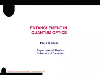
ENTANGLEMENT IN QUANTUM OPTICS. Paolo Tombesi. Department of Physics University of Camerino. OUTLINE. Introduction-definition of entangled states The Peres’ criterion for separability of bipartite states Experimental realization A general bipartite entanglement criterion

E N D
ENTANGLEMENT IN QUANTUM OPTICS Paolo Tombesi Department of Physics University of Camerino
OUTLINE • Introduction-definition of entangled states • The Peres’ criterion for separability of bipartite states • Experimental realization • A general bipartite entanglement criterion • Continuous variable case • The Simon’s criterion for Gaussian bipartite states • One example of continuous variable bipartite Gaussian states • Tripartite continuous variable Gaussian states • Example of tripartite Gaussian states
entanglement: polarization of two photons or (H1 H2 ± V1 V2)/√2 (H1 V2 ±H2 V1 )/√2 These are the so-called Bell states () and () In general, for a bipartite system, it is separable 12=i wiri1ri2 wi ≥ 0 i wi =1 i.e. it can be prepared by means of local operations and classical communications acting on two uncorrelated subsystems 1 and 2 Simple criterion for inseparability or entanglement was derived by Peres (PRL 77, 1413 (1996)
O x Given an orthonormal basis in H12 = H1 H2 the arbitrary state of the bipartite state 1+2 is described by the density matrix ( 12 )m,n (Latin indices for the first system and Greek indices for the second one). To have the transpose operation it means to invert row indices with column indices ( 12 )n ,m The partial transpose operation (PT) is given by the the inversion of Latin indices (Greek) PT : ( 12 )m,n ( 12 )n,m ( T112 )m,n It easy to prove that the positivity of partial transpose of the state is a necessary condition for separability. i.e. 12 separable T112≥ 0 We ask if the operator T112 is yet a density operator i.e. Tr (T112 ) = 1 and T112 ≥ 0 It easy to prove this because the transposition does not change the diagonal elements, Thus the Trace remains invariant, and the positivity is connected with the positivity of the eigenvalues of the matrix, which do not change under transposition. Then the violation of the positivity of the partial transpose is a sufficient criterion for entanglement T112 < 0 12 entangled In 2x2 and 2x3 dimension for the Hilbert space 12 separableT112≥ 0 Horodecki3 Phys Lett A 223, 8 (1996)
Non-linear crystal Pump laser Type I Type II
Pump Laser @405nm Phase Matching TYPE II 810nm Extraordinary y Ordinary 810nm 0.05 x 0.0 -0.05 0.0 0.05 -0.05 ((2)) NLC Laser beam Aperture Dichroic Mirror Polarization Entanglement | > = | H V > + e i| V H >
O x Let us consider a bipartite system whose subsystems, not necessarily identical, are labeled as 1 and 2, and a sepseparable state on the Hilbert space Htot = H1 H2. From the standard form of the uncertainty principle, it follows that every state on Htot must satisfy < ( u )2> < ( v )2> ≥ | a1b1< C1> + a2b2< C2>|2 4 We shall derive a general separability criterion valid for any state of any bipartite system. sep=i wiri1ri2 wi ≥ 0 i wi =1 Let us now choose a generic couple of observables for each subsystem, say rj, sj on Hj (j = 1, 2), Cj = i [rj , sj ] , j = 1, 2 Cj is typically nontrivial Hermitian operator on the Hilbert subspaces. Let’s define two Hermitian operators on Htot u = a1r1 + a2r2 , v = b1s1 + b2s2 where aj , bj are real parameters
For separable states the followingTheorem holds sep < ( u )2> < ( v )2> ≥ O2 With O= ( | a1b1| < O1> + | a2b2| < O2> ) /2 < Oj> = kwk< Cj >k < Cj >k = Tr [Cj k j] i.e. the expectation value of operator Cj onto k j From the definition of < ( u )2> and sep it is easy to see that Proof : < ( u )2> = kwk[ a12 < ( r1(k))2>k +a22 < ( r2(k))2>k] + kwk< uk>2 - (kwk< uk>)2 With rj(k)= rj - < rj>kthe variance ofrjonto the statekj The same for < ( v )2> For the Cauchy-Schwartz inequality kwk < uk>2 ≥(kwk < uk>)2 the last two terms in < ( u )2> are bound below by zero Follows < ( u )2> ≥kwk[ a12< ( r1(k))2>k +a22 < ( r2(k))2>k] and < ( v )2> ≥kwk[ b12 < ( s1(k))2>k +b22 < ( s2(k))2>k]
aj2< ( rj(k))2>k+ bj2 < ( sj(k))2>k ≥ aj2< ( rj(k))2>k + bj2 |< Cj>k |2 ≥ 4 < ( rj(k))2>k √ |ajbj| |< Cj>k | (min f(x) = 1x + 2 /x fmin = 2√1 2) Finally < ( u )2> + < ( v )2> ≥ 2√O O2 < ( u )2>≥ < ( v )2> Given any two real non negative numbers and < ( u )2> + < ( v )2> ≥kwk[a12< ( r1(k))2>k + b12 < ( s1(k))2>k + + kwk[a22< ( r2(k))2>k]+b22 < ( s2(k))2>k] Furthermore, by applying the uncertainty principle to the operators rj and sj on the state k j, it follows That has to be satisfied for any and positive, thus maximizing g(x) = 2 x O - x2 < ( v )2> for x > 0
The Duan et al. criterion (the sum criterion) Phys. Rev. Lett. 84, 2722 (2000) is a particular case of sep < ( u )2> < ( v )2> ≥ O2 O2 < ( v )2> Then < ( u )2> + < ( v )2> ≥ + < ( v )2> ≥ 2O O2 < ( u )2>≥ < ( v )2> Connection with other criteria Indeed, if we pose = = 1 in < ( u )2> + < ( v )2> ≥ 2√O We get < ( u )2> + < ( v )2> ≥ 2O however The last inequality holds because of the function (min f(x) = 1x + 2 /x fmin = 2√1 2) Giovannetti et al. Phys. Rev. A 67, 022320 (2003)
[X() , P() ] = i With Continuous variables A single qubit forms a 2-dim Hilbert space, a single quantum mechanical oscillator (i.e. single mode of the electromagnetic field or an acoustic vibrational mode) forms an ∞ - dim Hilbert space. This system can be described by observables (position and momentum), which have a continuous spectrum of eigenvalues. We will refer to this system as a continuous variable system (CV) .One can introduce the so-called rotated quadratures for the CV system X() = ( a e- i + a+ei)/√ 2 P() = ( a e- i - a+ei)/i √ 2 = X( +/2 ) A single mode of the e.m. field in free space can be written as E (r,t) = E0[X cos (t - kr ) + P sin ( t - kr )] in phase out of phase
O x N Passing to N modes the state H An arbitrary single mode state can be associated, by a 1 to 1 correspondence, to a symmetrically ordered characteristic function = R +i I () = Tr [ D() ] D() = exp( a + - * a ) = exp i √2(I x- R p ) With x and p position and momentum, or quadratures, of the CV mode The Wigner function W() of the state is related to () by an inverse Fourier Transform W() = - 2 ∫d2 exp( - * + * ) () () = ∫d2 exp( * - * ) W() Where the complex amplitude = R + i I represents the coherent state |> in the phase space. The W-function becomes W(1… N) = - 2N [k∫d2 k exp( - kk* + k* k )] (1.. N)
To the k-th mode we associate the complex variable k = kR +i kI which is Represented by the vector ( )=k real R2(k = 1,..,N) kI -kR In terms of the real variables ( T1,…..,TN) T R2Nthe arbitrary N-mode Gaussian characteristic function takes the form () = exp ( - TV + idT ) The corresponding N-mode Gaussian W-function by the inverse F-T is: exp( -1/4 dTV -1d) exp ( - T V-1 + dT V-1 ) W() = 2 √2 N√det V We shall consider N modes Gaussian states with the characteristic function (1,…., N) Gaussian as it is the W-function W(1,…,N) Where d R2N and V is a 2N x 2N real, symmetric strictly positive matrix V = V T V > 0 T (x1,p1,….,xN,pN) R2N Define a 2N-dim phase space
(-10) 0 1 N Introducing the N-mode symplectic matrix I(N)= Ii Ii = 1 V is the correlation matrix (CM) of the N-mode state Vnm = ( n m + m n) /2 (n,m = 1,2,….,2N) m= m - < m > d = < > is the displacement of the state Both d and V are measurable quantities defined for every N-mode state When the state is Gaussian it is fully characterized by these two quantities Gaussian ( V, d ) The CM expresses the covariance between the position and momentum quadratures (in-phase and out-of-phase) of the state . It must respect the uncertainty principle < ( xk ) 2 > < ( pk’ ) 2 > 1/4 k k’ (k,k’ = 1,..,N) The uncertainty principle readsV + i I(N)/2 o
Then the PT implies V V AB separable V +i I(2)/2 o V > 0 CV entanglement Simon (Phys. Rev. Lett. 84, 2726 (2000) showed how to extend the Peres criterion for separability to the CV case. Consider a bipartite CV state AB and introduce its phase space representation through the W-function W()T ( xA, pA, xB, pB) the PT operation on the state AB in HAB is equivalent to a partial mirror reflection of W()in the phase space PT : AB PT(AB ) W() W() with diag (1,1,1,-1) PT is a local time-reversal which inverts the momentum of only one subsystem (B in our case) The extension to CV of the Peres criterion is: AB separable W() is a genuine W-function genuinemeanscorresponding to a physical state A genuine W-function implies a genuine V CM i.e. AB separable Vis a genuine CM where V is the CM ofW()
A C 0 1 if V is of the form implies ( ) ( ) CT B -1 0 Where J = det A + det B o det A det B + ( 1/4 - |det C|)2 - Tr (AJCJBJCTJ) - 4 is the one-mode symplectic matrix AB(Gaussian) separable PT(AB) o This is the Simon’s criterion The condition AB separable V +i I(2)/2 o In the case of two-mode Gaussian states, the positivity of PT represents a necessary and sufficient condition for separability, i.e.
Generation of CV bipartite entangled state b2 Consider a beam splitter described by the operator B(,) = exp/2(a+1a2 e i - a1a+2 e-i ) a1 b1 where the transmission and reflection coefficients are t = cos /2 r = sin /2 while is the phase difference between the reflected and transmitted fields a2 If the input fields are coherent states we have B(,)| 1 >1)| 2 >2 = B(,)D1(1)D2(2)|0 >1)|0 >2 = D() = exp( a+- *a ) D1(1cos /2 + 2e i sin /2) D2(2cos /2 - 1e -i sin /2)| 0 >1|0 >2= | 1t + 2 r e i >1| 2t - 1 r e -i >2 And are not entangled. When the input states are squeezed states we get: (with j= rj e -2i) B(,) S1(1)S2(2)|0 >1)|0 >2 = B(,) S1(1) B+(,) B(,) S2(2) B+(,) B(,) | 0 >1)|0 >2 = S1(r1 + r2e2i ) S2(r1 e-2i + r2) S12(r1 e-i - r2 ei ) | 0 >1)|0 >2 S12()=exp( - a1a2+ *a+1a+2)is the two-mode squeezing operator
S() | 0 >1| 0 >2 = exp(a+1 a+2 tanh r ) X exp - (a1 a2 tanh r ) | 0 >1| 0 >2 = √ 1 - ∑nn/2 | n >1| n >2 1 ( ) a+1 a1+ a+2 a2 + 1 cosh r = tanh2 r Applying the two-mode squeeze operator S() = exp - r( a+1 a+2- a1 a2) ( = r e 2i with = 0 is the squeezing parameter) to two vacuum modes | 0 >1| 0 >2 And using thedisentangling theorem of Collet (Phys. Rev. A 38, 2233 (1988)). The two-mode squeezed vacuum state is the quantum optical representative for bipartite continuous-variable entanglement.
An arbitrary two-mode Gaussian state AB can be associated to its displacement d and CM V (such associationis a 1-1 correspondence in the case of a Gaussian state). Since its separability properties do not vary under LOCCs, we may, first, cancel its displacement d via local displacement operators Dk( k = A,B), and then reduce its CMV to the normal form For the two-mode vacuum squeezed state we have
The best way to see that it is really entangled is to consider the Simon criterion. With the V matrix given in normal form the Simon’s separability criterion V + iI (2)/2 0 reads 4(ab - c2) (ab - c’2) (a2 + b2) + 2 |c c’| - 1/4 Applied to the previous CM gives 1/2 (cosh 4r)/2 that is never satisfied for r 0.
CV TRIPARTITE entangled states A tripartite state is composed by three distinguishable parties A,B and C We’ll consider the scheme introduced by Dür et al. PRL 83, 3562 (1999) According with their classification one has five entanglement classes
Let us consider the Gaussian state 1N , which is a bipartite state of 1 X N ( i.e. 1 mode at Alice site and N on Bob’s site) and V 1,N be its CM, the partial transposition is given applying 1 = I (the partial transpose at Alice). The extension to more dimensions of the Simon’s criterion was proved by Werner and Wolf PRL 86, 3658 (2001) and is based on the positivity of the partial transpose CRITERION A Gaussian state 1N of a 1 X N system is separable (with respect to the grouping A ={1} and B ={2,…..,N}) if and only if 1 V1N 1 + iI (N+1)/2 0 The classification is given then as: (V’K = KVABC K+iI (3)/2 K = A,B,C ) class 1 V’A 0, V’B 0, V’C 0 class 2 V’A 0, V’B 0, V’C 0 (permutation of A,B,C) class 3 V’A 0, V’B 0, V’C 0 (permutation of A,B,C) class 4 or 5 V’A 0, V’B 0, V’C 0
For small mirror displacements, in interaction picture H = –∫d2r P(r,t) x(r,t) P is the radiation pressure force and x is the mirror displacement (r is the coordinate on the mirror surface) x(r,t) Pirandola et al. J. Mod. Opt. 51, 901 (2004) (Loudon et al. 1995) BOB
w0 0-W 0+W Pinard et al. Eur.Phys. J. D 7,107 (1999) x(r,t)b e-i Wt + b+ei Wt)exp[-r2/w2] fundamental Gaussian mode Frequency W and mass M
parametric interaction generates EPR-like entangled states used in continuous variable teleportation rotation (BS) it might degrade entanglement RWA (neglecting all terms oscillating faster than W) quant-ph/02/07094 - JOSA B 2003 Heff = - ic(a1b - a1+b+) - iq(a2b+- a2+b) a1 @ w0-W and a2 @ w0+W
Dynamics is studied with the normally ordered characteristic function F(m,n,z,t=0) = e -nth|n|2 m,n,z corresponding toa1,b,a2 nth = average number of thermal excitations for modeb i.e. initially vacuum states for a1 and a2 and b in a thermal state
After an interaction timet the state is 1 b 2 = ∫ d2m ∫ d2 ∫ d2F(m,n,z,t) e -(||2+ |n|2+ ||2)D1(-m) Db(-) D2(-) Di= normally ordered displacement operators Di()= e-cie*ci • F(m,n,z,t) is the evolution of F(m,n,z,) which is still Gaussian • F(m,n,z,t) = e- V T xT = (m1,m2,n1,n2,z1,z2) We can now study the class of entanglement of the tripartite state 1 b 2 Werner & Wolf PRL 86, 3653 (2001)
It turns out that 1 b 2 is bi-separable with respect to b at interaction times t = p, 3p, 5p, …. i.e. 1 b 2 is a one-mode bi-separable state (class 2 entangled) In particular the tripartite state at these times can be written as the tensor product of the initial thermal state of the mirror and a pure EPR state for a1 and a2with squeezing parameter depending on / !!Radiation pressure could be a source of two-mode entangled states!!
At all other times the tripartite state 1 b 2is fully entangled (class 1) at any nth b a1 By tracing out one mode of the three we study the entanglement of a bipartite subsystem a2 We find that mode a2 and b are never entangled Modes a1 and a2 are entangled (extremely robust with respect to the mirror temperature nth) Modes a1 and b are entangled even though the region of entanglement is small and depends on nth
REFERENCES Braunstein and van Loock Quantum Information with Continuous Variables to appear in Rev. Mod. Phys. quant-ph/0410100