Stability analysis in an example system
Stability analysis in an example system. Direct substitution and Dead Time. System diagram. Consider a system that can be represented by a first order process with dead time. An example of this type of system might be a fertigation system. Block diagram.

Stability analysis in an example system
E N D
Presentation Transcript
BAE 3023 Stability analysis in an example system Direct substitution and Dead Time
System diagram BAE 3023 Consider a system that can be represented by a first order process with dead time. An example of this type of system might be a fertigation system.
Block diagram BAE 3023 The system with a proportional controller might be represented as: Let tp =3, t0 = 2, KL = 1, KP = 1,
Method of direct substitution BAE 3023 A transfer function relating the outlet concentration to inflow changes would be: What would the ultimate gain for the controller be? In order to simplify the equation, we can use a series approximation for the exponential.
Finding the characteristic equation BAE 3023 Pade’s approximation: Let tp =3, t0 = 2, KL = 1, KP = 1,
Direct substitution BAE 3023 To find the ultimate gain, substitute iw for s and solve for Kc and w For the real part: And the imaginary part: From the imaginary part: From the real part: Note:
Zigler-Nichols BAE 3023 Zigler-Nichols, Quarter amplitude decay tuning Table 7-1.1 in Smith and Corripio
Controller tuning parameters BAE 3023 • For a PID controller and quarter amplitude decay Ziegler-Nichols tuning: Table 7-1.1
For use in MATLAB BAE 3023 %MATLAB setup for the SISOTOOL to examine the system performance tp=3; %Set the process time constant kp=1; %Set the process gain t0=2; %Set the dead time for the process [num_delay,den_delay]=pade(t0,1); %Calculate the transfer function numerator %and denominator polynomials for an approximation of the dead time tf_delay=tf(num_delay,den_delay); %Define the dead time transfer function tf_2=tf([kp],[tp 1]); %Define the process transfer function without the dead time g2=tf_2*tf_delay; % Define the process transfer function with dead time g3=1; %Define the sensor transfer function gc=tf([1.4 2.4 1],[2.4 0]); %Define the controller transfer function sisotool(g2,gc,1,1); %Start the SISO tool with the process and controller transfer function %Use the analysis tool to test the systems response to step disturbances