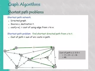
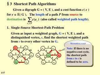
§3 Shortest Path Algorithms
Given a digraph G = ( V, E ), and a cost function c ( e ) for e E( G ). The length of a path P from source to destination is (also called weighted path length ). 2. v 1. v 2. 2. v 1. v 2. 4. 1. –10. 4. 1. 3. 10. 3. 2. 2. v 3. v 4. v 5. 2. 2.

§3 Shortest Path Algorithms
E N D
Presentation Transcript
Given a digraph G = ( V, E ), and a cost function c( e ) for e E( G ). The length of a path P from source to destination is (also called weighted path length). 2 v1 v2 2 v1 v2 4 1 –10 4 1 3 10 3 2 2 v3 v4 v5 2 2 v3 v4 v5 8 4 8 6 5 4 6 5 1 v6 v7 1 v6 v7 §3 Shortest Path Algorithms 1. Single-Source Shortest-Path Problem Given as input a weighted graph, G = ( V, E ), and a distinguished vertex, s, find the shortest weighted path from s to every other vertex in G. Negative-cost cycle Note: If there is no negative-cost cycle, the shortest path from s to s is defined to be zero. 1/17
§3 Shortest Path Algorithms v1 v2 v3 v4 v5 v6 v7 Unweighted Shortest Paths Sketch of the idea 0: v3 1 2 Breadth-first search 1: v1 and v6 2 0 3 2: v2 and v4 3: 1 3 v5 and v7 Implementation Table[ i ].Dist ::= distance from s to vi/* initialized to be except for s */ Table[ i ].Known ::= 1 if vi is checked; or 0 if not Table[ i ].Path ::= for tracking the path /* initialized to be 0 */ 2/17
§3 Shortest Path Algorithms v8 v7 v6 v5 v3 v2 v1 v9 v4 void Unweighted( Table T ) { int CurrDist; Vertex V, W; for ( CurrDist = 0; CurrDist < NumVertex; CurrDist ++ ) { for ( each vertex V ) if ( !T[ V ].Known && T[ V ].Dist == CurrDist ) { T[ V ].Known = true; for ( each W adjacent to V ) if ( T[ W ].Dist == Infinity ) { T[ W ].Dist = CurrDist + 1; T[ W ].Path = V; } /* end-if Dist == Infinity */ } /* end-if !Known && Dist == CurrDist */ } /* end-for CurrDist */ } If V is unknown yet has Dist < Infinity, then Dist is either CurrDist or CurrDist+1. T = O( |V|2 ) The worst case: 3/17
§3 Shortest Path Algorithms v1 v2 v3 v4 v5 v6 v7 DistPath v1 0 v2 0 v3 0 0 v4 0 v5 0 v6 0 v7 0 Improvement 1 2 void Unweighted( Table T ) { /* T is initialized with the source vertex S given */ Queue Q; Vertex V, W; Q = CreateQueue (NumVertex ); MakeEmpty( Q ); Enqueue( S, Q ); /* Enqueue the source vertex */ while ( !IsEmpty( Q ) ) { V = Dequeue( Q ); T[ V ].Known = true; /* not really necessary */ for ( each W adjacent to V ) if ( T[ W ].Dist == Infinity ) { T[ W ].Dist = T[ V ].Dist + 1; T[ W ].Path = V; Enqueue( W, Q ); } /* end-if Dist == Infinity */ } /* end-while */ DisposeQueue( Q ); /* free memory */ } 0 3 2 3 1 1 v3 v7 2 v1 v5 v4 2 v1 v2 3 v2 1 v3 v6 3 v4 v3 v1 T = O( |V| + |E| ) 4/17
§3 Shortest Path Algorithms Dijkstra’s Algorithm (for weighted shortest paths) Let S = { s and vi’s whose shortest paths have been found } For any u S, define distance [ u ] = minimal length of path { s ( vi S ) u }. If the paths are generated in non-decreasing order, then the shortest path must go through ONLYvi S ; u is chosen so that distance[ u ] = min{ wS | distance[ w ] } (If u is not unique, then we may select any of them) ; /* Greedy Method */ Why? If it is not true, then there must be a vertex w on this path that is not in S. Then ... if distance [ u1 ] < distance [ u2 ] and we add u1 into S, then distance [ u2 ] may change. If so, a shorter path from s to u2 must go through u1 and distance’ [ u2 ] = distance [ u1 ] + length(< u1, u2>). 5/17
§3 Shortest Path Algorithms Dist Path v1 0 0 6 8 9 5 1 3 3 2 v3 v7 v4 v1 v4 v4 v4 v1 v2 0 v3 0 v4 0 v5 0 2 v1 v2 v6 0 4 1 3 10 v7 0 2 2 v3 v4 v5 8 4 6 5 1 v6 v7 void Dijkstra( Table T ) { /* T is initialized by Figure 9.30 on p.303 */ Vertex V, W; for ( ; ; ) { V = smallest unknown distance vertex; if ( V == NotAVertex ) break; T[ V ].Known = true; for ( each W adjacent to V ) if ( !T[ W ].Known ) if ( T[ V ].Dist + Cvw < T[ W ].Dist ) { Decrease( T[ W ].Dist to T[ V ].Dist + Cvw ); T[ W ].Path = V; } /* end-if update W */ } /* end-for( ; ; ) */ } /* O( |V| ) */ /* not work for edge with negative cost */ Please read Figure 9.31 on p.304 for printing the path. 6/17
§3 Shortest Path Algorithms Implementation 1 V = smallest unknown distance vertex; /* simply scan the table – O( |V| ) */ Good if the graph is dense T = O( |V|2 + |E| ) Implementation 2 Home work: p.339 9.5 Find the shortest paths p.340 9.10 Modify Dijkstra’s algorithm V = smallest unknown distance vertex; /* keep distances in a priority queue and call DeleteMin – O( log|V| ) */ Decrease( T[ W ].Dist to T[ V ].Dist + Cvw ); Good if the graph is sparse /* Method 1: DecreaseKey – O( log|V| ) */ T = O( |V| log|V| + |E| log|V| ) = O( |E| log|V| ) /* Method 2: insert W with updated Dist into the priority queue */ /* Must keep doing DeleteMin until an unknown vertex emerges */ T = O( |E| log|V| ) but requires |E| DeleteMin with |E| space Other improvements: Pairing heap (Ch.12) and Fibonacci heap (Ch. 11) 7/17
§3 Shortest Path Algorithms Too simple, and naïve… Try this one out: 2 1 2 – 2 1 3 4 2 Graphs with Negative Edge Costs Hey I have a good idea: why don’t we simply add a constant to each edge and thus remove negative edges? void WeightedNegative( Table T ) { /* T is initialized by Figure 9.30 on p.303 */ Queue Q; Vertex V, W; Q = CreateQueue (NumVertex ); MakeEmpty( Q ); Enqueue( S, Q ); /* Enqueue the source vertex */ while ( !IsEmpty( Q ) ) { V = Dequeue( Q ); for ( each W adjacent to V ) if ( T[ V ].Dist + Cvw < T[ W ].Dist ) { T[ W ].Dist = T[ V ].Dist + Cvw; T[ W ].Path = V; if ( W is not already in Q ) Enqueue( W, Q ); } /* end-if update */ } /* end-while */ DisposeQueue( Q ); /* free memory */ } T = O( |V| |E| ) /* each vertex can dequeue at most |V| times */ /* no longer once per edge */ /* negative-cost cycle will cause indefinite loop */ 8/17
§3 Shortest Path Algorithms Signals the completion ofai ai ::= activity vj Index of vertex EC Time Lasting Time Slack Time LC Time Acyclic Graphs If the graph is acyclic, vertices may be selected in topological order since when a vertex is selected, its distance can no longer be lowered without any incoming edges from unknown nodes. T = O( |E| + |V| ) and no priority queue is needed. Application: AOE ( Activity On Edge ) Networks —— scheduling a project EC[ j ] \ LC[ j ] ::= the earliest \ latest completion time for node vj CPM ( Critical Path Method ) 9/17
§3 Shortest Path Algorithms 6 6 16 16 a0=6 a3=1 0 0 a6=9 a9=2 4 8 5 1 7 3 6 2 0 start 7 7 a1=4 18 18 a7=7 finish a10=4 4 6 a4=1 14 14 a2=5 a8=4 5 5 7 7 a5=2 Slack Time of <v,w> = 〖Example〗 AOE network of a hypothetical project 2 2 a11=0 3 Dummy activity Calculation of EC: Start from v0, for any ai = <v, w>, we have Calculation of LC: Start from the last vertex v8, for any ai = <v, w>, we have Critical Path ::= path consisting entirely of zero-slack edges. 10/17
§3 Shortest Path Algorithms 2. All-Pairs Shortest Path Problem For all pairs of vi and vj( i j ), find the shortest path between. Method 1 Use single-source algorithmfor |V| times. T = O( |V|3 ) – works fast on sparse graph. Method 2 O( |V|3 ) algorithm given in Ch.10, works faster on dense graphs. 11/17
s 2 3 1 a b 3 2 4 c d Determine the maximum amount of flow that can pass from s to t. 2 3 t §4 Network Flow Problems 〖Example〗 Consider the following network of pipes: source Note: Total coming in (v) Total going out (v) where v { s, t } sink 12/17
§4 Network Flow Problems s s s 2 3 1 a b a a b b 3 2 4 c d c d c d 2 3 t t t G Flow Gf Residual Gr 1. A Simple Algorithm Step 1: Find any path s t in Gr; Step 4: If (there is a path s t in Gr ) Goto Step 1; Else End. Step 2: Take the minimum edge on this path as the amount of flow and add to Gf; augmenting path Step 3: Update Grand remove the 0 flow edges; 13/17
§4 Network Flow Problems s 2 3 1 a b 3 2 4 c d 2 3 t G You are right! What if I pick up the path s a d t first? It is simple indeed. But I bet that you will point out some problems here… Uh-oh… Seems we cannot be greedy at this point. 14/17
§4 Network Flow Problems For each edge ( v, w ) with flow fv, w in Gf, add an edge ( w, v ) with flow fv, w in Gr. s s 2 3 1 a b a s b 3 2 3 2 3 2 3 2 4 1 c d a b c d 2 2 2 3 4 2 2 3 2 3 2 3 c d t t 2 3 3 2 G 3 Flow Gf 2 t Residual Gr 2. A Solution – allow the algorithm to undo its decisions 3 1 1 1 〖Proposition〗If the edge capabilities are rational numbers, this algorithm always terminate with a maximum flow. Note: The algorithm works for G with cycles as well. 15/17
§4 Network Flow Problems s 1 000 000 1 000 000 1 a b 1 000 000 1 000 000 t 3. Analysis ( If the capacities are all integers ) An augmenting path can be found by an unweighted shortest path algorithm. T = O( ) where f is the maximum flow. f · |E| Always choose the augmenting path that allows the largest increase in flow. /* modify Dijkstra’s algorithm */ T = Taugmentation * Tfind a path = O( |E| log capmax) * O( |E| log |V| ) = O( |E|2 log |V| ) if capmax is a small integer. 16/17
§4 Network Flow Problems Always choose the augmenting path that has the least number of edges. Home work: p.341 9.11 A test case. T = Taugmentation * Tfind a path = O( |E| ) * O( |E| · |V| ) /* unweighted shortest path algorithm */ = O( |E|2 |V| ) • Note: • If every v { s, t } has either a single incoming edge of capacity 1 or a single outgoing edge of capacity 1, then time bound is reduced to O( |E| |V|1/2 ). • The min-cost flow problem is to find, among all maximum flows, the one flow of minimum cost provided that each edge has a cost per unit of flow. 17/17