Realignment of Curves: Principles and Methods for Track Maintenance
610 likes | 726 Vues
Learn about the importance, objectives, and criteria of curve realignment, along with the string lining method's basic principles and procedures for track maintenance. Understand the principles of versines and the calculation of slews in curve alignments.

Realignment of Curves: Principles and Methods for Track Maintenance
E N D
Presentation Transcript
REALIGNMENT OF CURVES Prakash Kadiya. Sr. Inst. Track-7. 74200 41154
WHY SLEW REQUIRED ? • Because curve geometry gets disturbed under passage of traffic as • Trains are not moving at equilibrium speed • Large horizontal forces on the rails due to slight variations in curvature and due to vehicle imperfections
WHAT IS MEANT BY ROC ? • Bringing the curve back to proper alignment • Doesn’t necessarily mean restoring to original alignment • Infinite number of curves are possible between same set of tangents
OBJECTIVES OF ROC • No abrupt variation of curvature or superelevation • Superelevation should be in proportion to the curvature • Solution shall be practical • Least slews and subject to obligatory points NOTE: In electrified territory, there is severe restriction of the maximum amount of slews which can be permitted
REQUIREMENTS OF REALIGNMENT • Local adjustments • Realignments of transitions • Complete realignment (?) • During laying • During up-gradation • During remodelling • During service
CRITERIA FOR ROC • Unsatisfactory running • Based on results of curve inspection • Station to station variation is the primary consideration • Service limits laid down in IRPWM • If values go beyond service limits at more than 20% stations—realign within a month • If the variation is only at few stations, local adjustments shall be done
CURVE INSPECTIONS • By AEN : At least one curve in section of each SSE/P Way every quarter • By SSE/P Way in charge and assistant: • : Once in 6 months by rotation EXCEPT * • : *On A & B routes once in 4 months (CS 140). • Results to be recorded in Proforma given in Annexure 4/5 of IRPWM & TMS.
REALIGNMENT REALIGNMENT BY STRING LINING METHOD
Method of determining the corrections to be made in the alignment of the curve, after measuring the versines and the rectification there after is called string lining operation. STRING LINING METHOD BASIC PRINCIPLES
STRING LINING METHOD PROCEDURE • Measurement of Existing Versines. • Consideration of Obligatory Point. • Determination of Revised alignment & • Calculate the SLEW. • Slewing the Curve In the FIELD.
1stPRINCIPLE • Also known as 1st property of Versine of any curve. • “The slewing a station on curve affects the Versines at the adjoining stations either side by half the amount in opposite direction .”
C D B b’ b A C’ bb’/cc’=Ab/AC Ab=AB (being large radius) bb’/cc’=AB/AC = C/2C=1/2 bb’= (-)CC’/2
2ndPRINCIPLE • “In curves, between same set of tangents, • for equal chord lengths the sum of • versines is constant.”
Similarly, in JKL, < MKJ = 2ϒ and in ∆ MIK, ∆= < MIK+<MKI i.e. ∆=(2∝+β)+(β+2ϒ) » ∆ = 2[∝+β+ϒ] » ∆/2 = [∝+β+ϒ], -- 2. By putting value of 2 in 1. ∴ ΣV = (c/2)*( ∆/2) = C* ∆/4 Proof • Vo = c/2 tan ∝ ≅ c/2 ∝ • V1 = c/2 tan β ≅ c/2 β • V2 = c/2 tan ϒ ≅ c/2 ϒ M ∆ J α γ V1 2γ 2α K β β I V2 V0 ∴ ΣV = Vo + V1 + V2 = (c/2)*∝ + (c/2)*β+(c/2)* ϒ = (c/2)*(∝+β+ϒ) ----- 1. γ α C H L C/2
COROLLARY TO 2nd PRINCIPLE • “The chord length being equal, the sum total of the existing versines should be equal to the sum total of the proposed versines.”
3rd PRINCIPLE • “First summation of versines represents the area of versine diagram (in station distance units) • Summation means the sum of all the items above a certain station in the table
V0 Versine Diagram Vn Vn-3 Vn-2 Vn-1 V1 V2 V3 V4 If station to station distance is taken as unit, Area of each histogram segment= Ordinate at center i.e., V0, V1, V2, …., Vn-1 etc Total Area of the versine diagram= Sum of areas of each histogram segment = V0 + V1 + V2 + …. + Vn-1 Lever Arm for each histogram segment= n-station number • Moment of versine diagram about station n= n* V0+(n-1)* V1+ (n-2)V2+ ….. + 2* Vn-2+ Vn-1
4th PRINCIPLE • “Second summation of versines represents the moment of versine diagram about the last station ( in station distance units).”
V0 Moment of Versines around last Station Vn Vn-3 Vn-2 Vn-1 V1 V2 V3 V4 If station to station distance is taken as unit, Area of each histogram segment= Ordinate at center i.e., V0, V1, V2, …., Vn-1 etc Total Area of the versine diagram= Sum of areas of each histogram segment = V0 + V1 + V2 + …. + Vn-1 Lever Arm for each histogram segment= n-station number • Moment of versine diagram about station n= n* V0+(n-1)* V1+ (n-2)V2+ ….. + 2* Vn-2+ Vn-1
5th PRINCIPLE • Twice the second summation of the difference of proposed and existing versines up to a point gives the slew at a station. 2 * (SS OF Vp - Ve @ STN) GIVES SLEW OR • “The second summation of Versine difference represents half the slew at any station”
3’ 3x2V0 K 2x2V1 L 2xV2 M 2’ 3 N 2x2V0 G 2V1 H I V2 J 2 1’ • STN -1,0,1,2,3. AB TANGENT & BK EXTENTION. • E,I,N => 1,2,3 ON CURVE.AE IS CHORD FOR VERSINE @ 0. • BI & EN CHORD FOR STN 2 & 3. • BEHL JOINS STN 0 & 1 & FURTHER, EIM JOINS 1,2 & … • @ 0,Ve = V0. ABC & ADE, AD = 2 STN, AC = 1. DE = 2BC. • FURTHER BDF & BGH, BG = 2 BD. • GH = 2DE, GH = 2 * 2 * V0. D E 1 2xV0 V1 F 0 B V0 The offset from straight for the station no n: 2*n*V0+2*(n-1)V1+2*(n-2)V2+ … + 2*Vn-1 C -1 A
The solid curve represents curve as measured in field. Let the dotted line represent the desired geometry of the curve. Now the offset of the existing (solid) curve form straight is given by twice the second summation of the existing versines. Whereas the offset of the proposed (dotted) curve from straight is given by twice the second summation of the proposed versines. This means that if we calculate twice the difference of second summations of the existing and proposed versines,
COROLLARY TO 5TH PRINCIPLE • The second summation of the difference of proposed and existing versines at first and last stations shall be zero. • Means there should not be any residual slew value, if any, than should be distributed through correcting couple .
PRINCIPLES APPLIED IN ROC • Existing versines are available from measurements and the solution has to be ‘proposed’ • Take the difference between the existing and proposed versines and then work out first and second summation • The second summation of versine difference at the first and the last station should be zero. [Slew at the first and last stations shall be zero] • The first summation of versine difference shall be zero at last station • ROC AS DONE IN FIELD IS CALLED “STRING LINING OPERATIONS”
STEPS IN STRING LINING OPERATION • Survey existing versines • Find sum of existing versines and get an idea of the average versines • Propose new versines for the curve according to the principles : • Sum of existing versines = Sum of proposed versines • Uniform rate of change of versine in transition portion • Uniform versine over circular portion
STRING LINING METHOD--OPERATIONS • Workout Versine Difference (vp-ve) • Workout First Summation of Versine Difference • FS at last station shall be zero • Workout Second Summation of Versine Difference • Value at first and last station shall be zero
Station Msd. Ve Prop. Ve
STEPS IN STRING LINING OPERATIONS • If SS at last station is non-zero, apply Correcting Couple so that SS at last station becomes zero • Workout FS,SS for CC • Add the SS for original Versine difference and the SS for the correcting couple. • Workout Resultant Slew (These slews are to be actually applied in field) • Workout Resultant Versines, for checking the slews (= vp+ CC)
Correcting Correcting
Use of correcting couple • There is a residual second summation of versine difference is +104 at the last station, it means that the second summation of existing and proposed versines are not equal. • This also means that centre of gravity of existing versine diagram does not coinside with the proposed versines. • The correcting couple which is small correction in the proposed versine diagram.
Principles of choosing correcting couple. • These are equal and opposite. • If the residual second summation of versine difference at the last station is positive, a negative correction is applied at the initial stations of the curve and positive correction is applied at the later station of the curve. So SS will be negative. Similarly vice versa for negative residual value.
Principle contd.. • The correcting couple disturbed trapezoidal distribution of the proposed versines , and consequently correction shall be as small as possible in value. • If the correction are applied farther apart , the second summation of the correcting couple will be higher.
Correcting Correcting
Correcting Correcting
SHORTCOMINGS IN METHOD • Difficult to decide proposed versines, especially when the stations are more. • There is no way to know if the length of existing curve was ok • Curve may increase or decrease in length during service • affects assumed proposed versines • Correct beginning of curve is not known
OPTIMISATION METHOD • Optimization • By finding out the • correct beginning and end of the curve • Correct length of curve • Control by keeping slew at centre of curve as zero. • Used in computer programs as calculations tedious by hand.
Improper choice of Beginning of Curve: When the proposed Versine chosen happens to be correct but the BC chosen is not correct, it results in heavy residual slew at the end,
Improper Choice of versine: When the BC chosen is correct but the proposed versine chosen is not correct, it results in heavy slews outward or inward over the entire curve. The effect of different versine readings is shown
1. Find the Center of Curve :- It is not the physical center of curve length but it’s X coordinate of the center of the Versine diagram of gravity. CG of existing VD can be determined by MOMENT OF THE VD ABOUT LAST STATION AREA OF VD. To ascertain the value of CC W. R. T. first station, We have to Deduct CG found from last station (n) SS OF Ve UPTO LAST STN FS OF Ve UPTO LAST STATION Centre of Curve =
2. FIND OFFSET FROM TANGENT AT CC for V existing It can be found out by the principle of Second Summation as discussed. It is given by SS of Ve at that station. If CC happens to be fall between two stations, by interpolating SSs of adjoining stations, offset can be calculated. 3. FIND OFFSET FROM TANGENT AT CC for Vproposed. It is desirable to have same CC, we have to equate OFFSETs. We have found OFFSET for CC (Ve). & we can find CC of Vp By considering Equivalent Circular Curve.(ECC) ECC is the proposed curve does not having TL.
Let the Length of proposed ECC is N units. Let the Uniform Versine be the V. Let the TL length be L. If T is the tangent length up to CC, for ECC ,the OFFSET @ Centre of curve Oc = square (T) / 2*R. Since the actual proposed curve having TL @ either ends, The curve will shift inwards by ‘S’, due to introduction of TL. Offset @ CC = square (T) / 2*R + square (L) / 24 R.
4. Equate the OFFSETS AT CC OF existing & proposed Curve.:- V = C2 / 8*R. C = 2 STATIONS. V = 22 / 8*R=1/2. For Rly curve R is large & hence TL T = ½ Curve Length = N/2. Now, Put the values in eq. OFFSET AT CC = T2 / 2R+L2 / 24R, = VN2 /4 + VL2 /12 Due to the Versine designed by slope method above equation will Be slightly altered, OFFSET @ CC = VN2 / 4+V(L2 - 4)/12. = V2 N2 + V (L2-4) VERSINE OF ECC = V*N HENCE, 4V 12 NOW, V*N = FSVe i.e. OFFSET @ CC = (FSVe)2 + V (L2-4) 4V 12
5. FIND OUT LENGTH OF CURVE :- V * N = FSVe i.e. N = FSVe / V. LENGTH OF PROPOSED CURVE CAN BE CALCULATED BY ADDING THE DESIGNED TL IN STATION UNITS TO THE CIRCULAR CURVE. N’ = N + L 6. BEGINNING & END OF CURVE :- BC = CC - AND EC = CC + N+L 2 N+L 2 7. VERSINE PROPOSED :- V IN CIRCULAR PORTION WILL BE V AND SLOPE V/L .
FORMULA FOR OPTIMISATION Actual Offset at CC= Offset in equivalent circular curve at CC + shift = Oc + S = T2/2R + L2/24R; Now, T = N/2; And V=C2/8R; C=2 stn units; i.e. V=1/2R = V*N2/4 + V*L2/12 =(VN)2/4V + VL2/12 Due to correction near the ends of transitions: Actual Offset at CC= ~ (FSVe)2/4V+ V (L2-4)/12
OPTIMISATION PROCEDURE • Workout FS and SS of existing versine (ve) • Find out chainage of CC, x = N-SS upto N / FS upto N • Find out offset at x from table of SS by interpolation • Assume length of transition L • Find out Vby solving equation: Actual Offset at CC= (FSVe)2/4V+ V (L2-4)/12