Smooth Curve Designing with Polyloop Transformations and Subdivisions
Explore polyloops design paradigm, algorithms for smooth curve conversion, and subdivision schemes. Understand tangent and curvature estimation for smooth rendering.

Smooth Curve Designing with Polyloop Transformations and Subdivisions
E N D
Presentation Transcript
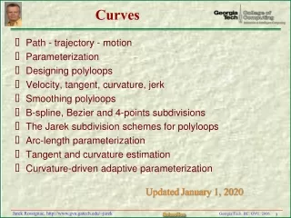
Curves • Path - trajectory - motion • Parameterization • Designing polyloops • Velocity, tangent, curvature, jerk • Smoothing polyloops • B-spline, Bezier and 4-points subdivisions • The Jarek subdivision schemes for polyloops • Arc-length parameterization • Tangent and curvature estimation • Curvature-driven adaptive parameterization Updated January 1, 2020
How to specify a curve? • Implicit (equation): x2+y2=r2 • Not convenient for walking on the curve • Parametric (function): P(s) = ( r cos(s) , r sin(s) ) • Polyloop: cycles of edges joining consecutive points (vertices) • Not smooth,unless you use lots of vertices • Subdivision: result to which a subdivision process converges • Procedural: snowflake, fractal, subdivision… V2 V3 V1 V5 V4 V0
It is all about curves Points, vectors curves Shapes Motions Animated shapes
Outline • We will talk about polygonal loops (polyloops) in the plane • We will discuss algorithms to transform them into smoothcurves • We want to support an intuitive design paradigm: • A designer adjust the vertices of the control polygon (polyloop) • The corresponding smooth curve is regenerated automatically • The effect of an adjustment should be local and predictible • We will look at several subdivision schemes for converting a control polyloop into a smooth curve • We will study their properties and look at several applications • Smooth rendering, culling and clipping • Computing intersections, areas • We will extend these results to • 3D curves • Surfaces • Animations
Geometry review • The constructions and algorithms that follow are formulated in terms of simple geometric constructions that involve points, vectors, and operators. • We will first • provide an overview of these fundamental concepts • propose a few convenient operations • define our notation
P=(4,3) J O I Points • A point is a location in space (zero dimensional entity) • Initially space will the plane (later we will go 3D) • How to represent a point P? • Assume a known origin O and two orthogonal directions I and J (unit basis vectors) • Represent P by its two coordinatesP=(x,y) where P=O+xI+yJ • To get to P: • start at O, • walk x units along the direction I, • then y units along the direction J • REMEMBER THIS EXPLANATION! • It is the key to understanding • Coordinate systems • Graphic transformations • Animations
Vectors • A vector is either a direction or a displacement between two points (locations). • We will also use vectors to represent forces and velocities. • A vector is often represented by its coordinates: V=(x,y) • Please do not confuse points and vectors! • A direction is a unit vector. It may represent • the direction of a ray from the eye through a pixel • the direction towards the light from a point on a surface • the tangent to a curve at a specific point • a basis vector for expressing the coordinates of points • Displacement vectors may be computed as point subtractions • Let V be the displacement vector from A=(xA,yA) to B=(xB,yB) • V may be denoted B–A, or for short AB • Its coordinates may be computed as V =(xB–xA, yB–yA) • Hence, given O, a point P corresponds to the vector OP • Assuming that the coordinates of the origin O are (0,0)
V+V’ V’ V –V Operations on vectors • Consider two vectors: V=(x,y) and V’=(x’,y’) • Scaling vectors sV= (sx,sy) • Reversing a vector: –V=(–x,–y) • Adding vectors V+V’= (x+x’,y+y’) • Subtracting vectors V–V’= (x–x’,y–y’) • What do the coordinate mean? • Consider a basis of two orthogonal unit vectors I and J • V=(x,y) means that V=xI+yJ • Walk x units along I and y units along J
U U.away(V) U.along(V) V “Advanced” vector operators and notation • Let V=(x,y) and U=(a,b) • Length of V is computed by V.norm=sqrt(x2+y2) • Unit length vector obtained by normalizing V: V.unit=(1/V.norm)V, • Orthogonal vector (rotating V ccw by 90 degrees) V.left=(–y,x) • Cascading “.” notation (left-to-right): V.left.norm=(V.left).norm • Dot product: UV=ax+by (a scalar!) • When V.norm=U.norm=1, then UV is the projection of U onto V • Proof: write U=cV+dV.left=(cx–dy,dx+cy), solving for c with x2+y2=1 yields c=ax+by • Otherwise: UV is the projection of U onto V scaled by the length of V • UV = U.norm*V.norm*cos(angle(U,V)) • Properties of dot product • UV = VU • (–U)V = –(VU) • UV = 0 implies that they are orthogonal or one has zero length • Tangential and orthogonal decomposition U with respect to a vector V: • along V: U.along(V):=(UV.unit)V.unit • awayfrom V: U.away(V):=U–U.along(V)
Walking along an edge • Consider an edge from point A to point B: denoted Edge(A,B) • You can use a parameter, s, in [0,1] to identify any point P(s) on it P(s)=A+sAB • This is the proper notation: start at A and move by s along vector AB • For convenience, we often use another equivalent notation: P = A+s(B–A) = (1–s)A+sB • Note that P(0)=A and P(1)=B 1–s B s P(0.6) A
P P AP B AP H B H A A s=1.4 s=0.6 Closest point on an edge • Consider Edge(A,B) and a point P in the plane • Compute the point C of Edge(A,B) that is the closest to P • First compute the parameter s of the orthogonal projection H of P on Edge(A,B) • Then test it against [0,1] and decide Procedure project (A,B,P) { s:=APAB/ABAB; # assuming AB IF 0<s<1 THEN RETURN A+sAB ELSE IF s<0 THEN RETURN A ELSE RETURN B } To compute closest point to P on polyloop: Compute it for all edges and take closest
Arclength of an edge • Write the procedure L(A,B) that returns the arclength of edge (A,B)
Total arclength of a polyloop • Write the procedure L(C) that returns the total arclength of polyloop with vertices C[i], for i = 0, 1, … n
Terminology (for lack of a better one) • A path is a parameterized curve (2D or 3D) • A point (of an object) may follow a curve • The path indicates where we are along the curve at each moment of the animation • The orientation of the object is not defined (could be pure translation?) • A motion defines the evolution of a pose • Position and orientation of the local CS or object(s) defined in it • A trajectory is a motion defined by a path • The orientation is defined by the tangent to the curve • …and bi-tangent in 3D…
Curve and path Given a path P(t), what is the curve traced by P(t)? Union of all points P(t) What if P(t) starts at A, moves a few times back and forth along the segment (A,B) then finishes at B? The path is complicated The curve is trivial
Motivation • Assume that you have a polyloop P path defined by sampling positions Pi or produced by subdividing a control polygon L • In general, the vertices of P are not uniformly spaced • Their spacing may reflect the animator’s desire to slow down near turns or at specific places • or it may be the undesired side effect of data acquisition or creation • We may want to re-parameterize P to obtain a path P’ that moves at constant speed if you use s(P’i,t,P’i+1) on each segment • Then, you can warp time (as in project P1a) to impose your own speed profile, independently on the original sampling of P
4-pt subdivision slower faster resampling constant speed Example where resampling is needed Subdivision of a bad control polygon
P(1)=P(0) t P(.5) Arclength reparameterization • Write the procedure for computing a point on the polyloop that corresponds to parameter t in [0,1] • Demonstrate it by animating a point at constant speed
Research challenge!!! Given a polyloop P, place an ordered set of k points along P so that each point is at the same Euclidean (shortest) distance to its two neighbors. Is is always possible? Is there a deterministic algorithm? Would an iterative algorithms always converge?
Polygon area calculation: 2 methods • Sum of signed areas of triangles, each joining an arbitrary origin o to a different edge(a,b) • SUM (oaob) for each edge (a,b) • uv is the dot product of v with the the vector obtained by rotating u by 90° • Sum of signed areas of trapezoids between each oriented edge and its orthogonal projection (shadow) on the x-axis y by b ay a x ax bx area(a,b):=(ay+by)(bx–ax)/2
Area implementation float area () { float A=0; for (int i=0; i<vn; i++) A+=trapezeArea(P[i],P[this.in(i)]); return(A); } float trapezeArea(pt A, pt B) {return((B.x-A.x)*(B.y+A.y)/2.);}
Centroid of polygonal region • Weighted sum of centroids of trapezoids • Weight = signed area of trapezoid / total area
Centroid of trapezoid Any line through centroid cuts shape in 2 parts with same moment x = 0∫1 sy(s)ds / 0∫1 y(s)ds, with y(s)=a+s(b–a) x = 0∫1 (b–a)s2 + as ds / 0∫1 (b–a)s +a ds x=(a+2b)/(3(a+b)) Similar derivation: y= (a2+ab+b2)/(3(a+b)) y b a (x,y) x 0 1
Implementation of centroid pt barycenter () {G.setTo(0,0); for (int i=0; i<vn; i++) G.addScaledPt( trapezeArea(P[i],P[this.in(i)]),trapezeCenter(P[i],P[this.in(i)])); G.scaleBy(1./this.area()); return(G); } pt trapezeCenter(pt A, pt B) { return(new pt( A.x+(B.x-A.x)*(A.y+2*B.y)/(A.y+B.y)/3., (A.y*A.y+A.y*B.y+B.y*B.y)/(A.y+B.y)/3.) ); }
Principal directions of polyloop • For a set of points sampled along the curve • Not the same as principal axes (second order inertia moments)
Implementation of principal direction void showAxis() {pt G=this.barycenter(); stroke(black); G.show(10); float xx=0, xy=0, yy=0, px=0, py=0, mx=0, my=0; for (int i=0; i<vn; i++) {xx+=(P[i].x-G.x)*(P[i].x-G.x); xy+=(P[i].x-G.x)*(P[i].y-G.y); yy+=(P[i].y-G.y)*(P[i].y-G.y);}; float a = atan(2*xy/(xx-yy))/2.; vec V= new vec(50,0); V.rotateBy(a); vec U = V.makeTurnedLeft(); for (int i=0; i<vn; i++) {vec W=G.makeVecTo(P[i]); float vd=dot(W,V); float ud=dot(W,U); if(vd>0) px+=vd; else mx-=vd; if(ud>0) py+=ud; else my-=ud; }; if(mx>max(px,py,my)) V.rotateBy(PI); if(py>max(px,mx,my)) V.rotateBy(PI/2.); if(my>max(px,mx,py)) V.rotateBy(-PI/2.); strokeWeight(1); stroke(black); V.showArrowAt(G); stroke(black,60); V.turnLeft(); V.showAt(G); V.turnLeft(); V.showAt(G); V.turnLeft(); V.showAt(G); }
Questions • Describe two techniques for testing whether a point q lies inside a polygon P • Describe two techniques for computing the area of a polygon P • Assume that you have a function fill_tri(a,b,c) that will visit all pixels whose center falls inside the triangle with vertices (a,b,c). Assume that each time the function visits a pixel, it toggles its status. Initially, all the status of each pixel is OFF. Explain how you could turn to ON the status of all pixels whose center falls inside a polygon P.
Motivation • Smooth curves and surfaces are used for aesthetic, manufacturing, and analysis applications where discontinuities due to piecewise linear approximations would create misleading artifacts. • Designers like to specify such curves by adjusting a control network with only a few vertices • How to go from a crude 2D control polyloop (black) to a smooth curve (red)? • Suggestions?
compromise Different requirements smooth interpolating
Operators on polyloops Simplification Subsampling Smoothing Denoising Subdivision Refinement Adding noise
Motivation for curve smoothing • Smooth curves and surfaces are used for aesthetic, manufacturing, and analysis applications where discontinuities due to triangulated approximations would create misleading artifacts. • Smooth curves may be used to design trajectories and paths for movingobjects and cameras in animations. • Designers like to specify such curves by adjusting a crude control polygon with only a few vertices • How to go from a crude control polygon (black) to a smooth curve (red)? • Suggestions?
Local curve analysis • We first investigate local differential properties of a polyloop L • to measure forces, compare schemes, adjust speeds… • … but these are trivial for a polyloop • straight line segments (zero curvature) • not differentiable at vertices (infinite curvature) • So… we really want the properties of the smooth curve or path J defined by L • tangent, normal, acceleration, curvature, jerk • … but, we usually do not know J • it may be defined as the limit of a smoothing process • Therefore, we use discreteestimators for these properties
AB B V(B) L C A V(B) Velocity at a vertex: V(B)=(AB+BC)/2 • Let A,B,C,D,E… be consecutive vertices in L • AB, BC,… are the edges of L • J is the unknown smooth curve passing through the vertices • When traveling along J from A to B, it takes 1 sec. • Hence the average velocity vector for that segment is AB. • Hence the velocity at B is estimated as V(B)=(AB+BC)/2
AB B V(B) L C A V(B) Implementing V(B)=(AB+BC)/2 class vec { float x,y; vec average(vec U, vec V) {return(new vec((U.x+V.x)/2,(U.y+V.y)/2)); }; void unit() {float n=sqrt(sq(x)+sq(y)); if (n>0.000001) {x/=n; y/=n;};}; … class pt { float x,y; vec vecTo(pt P) {return(new vec(P.x-x,P.y-y)); }; Write a method for the pt class that computes the velocity at point B vec velocity (pt A, pt C) {…}; tangent T(B) = V(B).unit()
N(B) B V(B) C A Normal at a vertex: N(B)=AC.left().unit() • The normal N(B) at B is the unit vector orthogonal to AC. • We pick the one pointing left: N(B)=AC.left().unit() class vec { float x,y; void left() {float w=x; x=-y; y=w;}; void unit() {float n=sqrt(sq(x)+sq(y)); if (n>0.000001) {x/=n; y/=n;};}; Write a method for the pt class that computes the normal at point B vec normal (pt A, pt C) {…};
B V(B) C g(B) A Acceleration at a vertex: g(B)=BC–AB • The acceleration at B is the velocity change g(B)=BC–AB • It is useful for computing forces during animation (dynamics) Write a method for the pt class that computes the acceleration at point B vec acceleration (pt A, pt C) {…};
Radius of curvature: r(B)=V2/(2ABN(B)) • The radius r(B) of curvature (sharpness of turn in the path) at B could be estimated as the radius of the circle through A, B, and C, but this approach yields unexpected results when the angle at b is acute. • I prefer to use the parabolic curvature, r(B)=V2/(2h), where V is the magnitude of V(B) and where h is the distance from B to the Line(A,C). • h=ABN(B) is the normal component of g(B) • It measures the centrifugal force • Curvature = 1/r(B) Write a method for the pt class that computes the r(B) at point B vec radiusOfCurvature (pt A, pt C) {…};
j(B,C) B C –g(B) g(C) g(B) A D Jerk: j(B,C)=AD+3CB It is the change of acceleration between B and C. It measures the change in the force felt by a person traveling along the curve j(B,C) = g(C)–g(B) = (CD–BC)–(BC–AB) = CD+CB+CB+AB = AB+BC+CD + CB+CB+CB = AD+3CB To show the second degree discontinuities in the curve, draw the normal component of j(B,C) at (B+C)/2
smoothing Smoothing a polyloop Given a polyloop L, we wish to move its vertices to produce a curve J that resembles L, but is “smoother” (less jerk?) Smoothing does not change the number of vertices, it only moves them
tuck(.5) tuck(.5) tuck(.5) tuck(.5) Tuck smoothing tuck(s) moves the vertices by executing the following two steps: • For each vertex B, compute M(B)=(BA+BC)/2 • A (r. C) is the previous (r. next) vertex in the cyclic order • Moving B to B+M(B) brings it to the average of its neighbors • For each vertex B, move B to B+sM(B) Repeating tuck(s) tends to eliminate sharp features, but shrinks the curve …
Avoid oscillations Keep s in [0,2/3] to avoid oscillations tuck(1) tuck(1)
Avoid shrinking: Tuck-tuck smoothing • Alternate tuck(s), which shrinks, and tuck(–s), which expands • untuck cannot recover the sharp features lost during the tuck
dual dual Tuck(1/2) = dual of dual • Tuck(.5) is the dual of the dual • refine introduces a new vertex in the middle of each edge • kill deletes the old vertices • dual = (refine, kill) • tuck(.5) = (dual, dual) refine kill
C(0) C(1) C(-1) M B D C(2) C(-2) A E M’ smoothing bulge M’M/3 Cubic fit tuck-tuck: (–A+4B+4D–E)/6 Compute a cubic polynomial curve, C(t)=at3+bt2+ct+d, through vertices A, B, D, E satisfying: C(–2)=A, C(2)=E, C(–1)=B, and C(1)=D We want to insert a point C=C(0)=d between B and E. Solve for d C(–2)=–8a+4b–2c+d=A and C(2)=8a+4b+2c+d=E yields A+E=8b+2d C(–1)=–a+b–c+d=B, and C(1)=a+b+c+d=D yields A+E=8b+2d A+E=8b+2d and A+E=8b+2d yields 6d=4(B+D)–(A+E) d = (–A+4B+4D–E)/6 = M+M’M/3, with M=(B+D)/2, M’=(A+E)/2) To insert such a cubic fit for each edge: tuck(2/6), tuck(–2/6) Note that 2/6=0.82, which may be unstable Move towards C
Smoothing vs subdivision • Smoothing should be performed when the desired curve has been densely sampled but the resulting polyloop has undesiredsharp features (acquisition noise, too many details, sharp changes in direction or curvature) • Subdivision refines the polyloop (adds more vertices). It should be performed when the polyloop is a crude outline of the desired curve. subdivision smoothing
Polyloop refine/smooth operators We will use the following operators: • r (refine) introduces a new vertex in the middle of each edge • k (kill) deletes the old vertices (those present before r) • d (dual) performs (r, k) • t (tuck) performs tuck(1/2), which is (d, d) • us (parameterized untuck) performs tuck(–s) • u (untuck) performs tuck(–1/2), same as u.5 Write a polyloops smoothing scheme using these
Quadratic uniform B-spline (r,d) Repeating (r,d) converges to a piecewise quadratic B-spline curve that interpolates the mid-edge points r rd rdrd rdrdrdrd
Cubic uniform B-spline (r,t) Repeating (r,t), which is (r,d,d) converges to a piecewise cubic B-spline curve that has second degree continuity (no jerk) rt rtr rtrt rtrtrt
2 B A 3 1 4 8 5 7 C D 6 Split&tweak B-spline subdivision • Given a control polygon, for example (A,B,C,D), repeat the following sequence of two steps, until all consecutive 4-tuples of control points are nearly co-linear. 1. “Split”: insert a new control point in the middle of each edge (2,4,6,8) 2. “Tweak”: move the old control points half-way towards the average of their new neighbors (1,3,5,7) • The polyloop converges rapidly to a smooth curve, which happens to be a cubic B-spline curve.
Can the limit curve self-intersect? • Can it self-intersect when P does not?

