Curves
Curves. Locus of a point moving with one degree of freedom Locus of a one-dimensional parameter family of point Mathematically defined using: Explicit equations Implicit equations Parametric equations (Hermite, Bezier, B-spline). Geometric Modeling of Curves.

Curves
E N D
Presentation Transcript
Curves • Locus of a point moving with one degree of freedom • Locus of a one-dimensional parameter family of point • Mathematically defined using: • Explicit equations • Implicit equations • Parametric equations (Hermite, Bezier, B-spline)
Geometric Modeling of Curves Computational Representations of a Curve for: • Data fitting applications • Shape representation (e.g. font design) • Intersection computations
Differential Geometry Characterization Frenet Frame Formulation • Use of tangent, main normal and binormal: T = P’(u)/ || P’(u) || B = P’(u) X P”(u) / || P’(u) X P”(u) || M = B X T • (T,M,B) is the Frenet frame; it varies its orientation as u traces the curve
Differential Geometry Characterization • Arc Length Parametrization: Assume that the magnitude of the derivative vector is 1. That implies that: P’(u) . P’(u) = 1; & P’(u) . P”(u) = 0 • Frenet-Serret formulas: T’ = M M’ = - T + B B’ = - M is the curvature is the torsion
Differential Geometry Characterization Intrinsic Properties • Curvature as a function of arc length: rate of change of tangent vector • Torsion as a function of arc-length: how much a space curve deviates from a plane curve or rate of change of binormal vector
Explicit Equations Y = f(x) • There is only one y value for each x value; not vice-versa • Easy to generate points or plot of the curves • Can easily check whether a point lies on the curve • Cannot represent closed or multiple-valued curves
Implicit Equations Can represent closed form or multiple-valued: f(x,y)=0 • Mostly deal with polynomial or rational functions • Implicits are a proper superset of rational parametric E.g. Line: Ax + By + C = 0 Conic: Ax2+ 2Bxy + Cy2 + Dx + Ey + F = 0 The coefficients determine the geometric properties
Parametric Equations of Curves P(u) = [x(u) y(u) z(u)] where x( ), y( ) and z( ) are polynomial or rational functions. The definition extends to N-dimensions • Usually the domain is restricted to u [0,1] or a subset of real domain • Each piece is a curve segment Q(u,v) = [x(u,v) y(u,v) z(u,v)] is a surface P( ) and Q( ) are vector valued functions Partials of P( ) & Q( ) are used to compute tangents and normals to the curves & surfaces
Parametric Equations of Curves • Model Space: x,y,z Cartesian • Parametric space: u,v space or parametric domain • Direct Mapping: Parametric => Model space • Involves function evaluation • Inverse mapping or Inversion: Given (x,y,z) compute u or (u,v) • Involves solving non-linear equations • Reparametrization: To change the parametric domain or interval used to define the curve
Advantages of Parametric Formulation • Allow separation of variables & direction computation of point coordinates • Easy to express them as vectors • Each variable is treated alike • More degrees of freedom to control curve shape • Transformations can be performed directly on the curves • Accommodate slopes without computational breakdown
Advantages of Parametric Formulation • Extension or contraction to higher or lower dimension is direct • The curves are inherently bounded when the parameter is constrained to a specified finite interval • Same curve can be represented by mulitiple parametrizations • Choice of parametrization, because of computational properties or application related benefits
Conic Curves Ax2+ 2Bxy + Cy2 + Dx + Ey + F = 0 has a matrix form P Q PT = 0, where P = [ x y 1], & Q = A B D B C E D E F P is given by homogeneous coordinates
Conic Curves • Many characteristics are invariant under translation and rotation transformation • These include, A + C, k = AC – B 2 , and the determinant of Q • The values of k and Q indicate the type of conic curve • Common conics are parabola, hyperbola and ellipse
Parametric Curves • Hermite Curves: based on Hermite interpolation; uses points & derivative data • Bezier Curves: Defined by control points which determine its degree; interpolates the first & last point; no local control • B-Spline Curves: piecewise polynomial or rational curve defined by control points; need not interpolate any point; degree is independent of the number of control points; local control; affine invariance