Measures of Community Diversity: Analyzing Species Richness and Distribution in Ecology
180 likes | 300 Vues
This resource provides an in-depth examination of community diversity metrics, focusing on species richness and individual distribution. It discusses various methodologies for estimating absolute richness, including sample-based and individual-based approaches. The Shannon Index and Simpson's Index are highlighted as tools for measuring diversity and evenness, while practical examples illustrate their use. Additionally, the importance of adequate sample size and area in community studies is emphasized, including techniques like rarefaction curves and confidence interval calculations.

Measures of Community Diversity: Analyzing Species Richness and Distribution in Ecology
E N D
Presentation Transcript
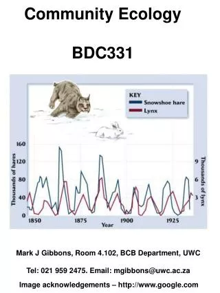
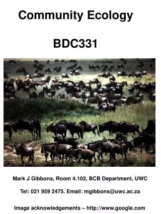
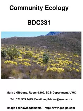
Community Ecology BDC331 Mark J Gibbons, Room 4.102, BCB Department, UWC Tel: 021 959 2475. Email: mgibbons@uwc.ac.za Image acknowledgements – http://www.google.com
B A COLOUR A B RED 18 41 LILAC 14 3 YELLOW 4 2 ORANGE 6 3 LIGHT GREEN 5 4 DARK BLUE 4 2 BLACK 9 7 APPLE GREEN 3 2 LIGHT BLUE 2 1 TOTAL 65 65 Description of Communities Guild Taxocene Measures of Community Diversity Species Richness - S Same Number Species – 9 Same Number individuals - 65 Different Distribution of individuals amongst species
Species Density Botanists Number of Species Observed Total Number of Individuals Counted Determining Species Richness Numerical Species Richness Sample-based Samples taken: all individuals within identified & counted Individual-based Individuals sampled sequentially Focus of Community Studies PROBLEM: Number of species reflects number of samples or individuals
COMMUNITIES vs SAMPLES
Species-Area or Accumulation Curves Asymptote considered to represent the number of species occurring in the community Issues of Sample Area or Number
There are a number of ways of determining this: Randomised 999 times Rarefaction Curves The absolute number of species likely to be found in the pool is obtained when the curve flattens out WHEN IDENTIFYING or COMPARING COMMUNITIES, ARE YOU INTERESTED IN ESTIMATING ABSOLUTE RICHNESS? DEPENDS ON THE QUESTION BEING ASKED
Effort (area or number of samples or individuals) is important STANDARDIZE a priori HOW?
Shannon Index (H’ ) ∑ H’ = - pi ln(pi) pi = Proportion of the ith species Varies between 1.5 and 4. Sensitive to the abundance of rare species Should ONLY really be used for datasets where absolute richness known – otherwise Brillouin Index Heterogeneity Measures Species Diversity Indices
( ) 1 N! ln = n1! n2! n3! n4! ...... N N = total number of individuals in the entire collection n1 = Number of individuals of species 1 n2 = Number of individuals of species 2 Best used where data not random Sensitive to the abundance of rare species ^ H ^ H can only use count data Brillouin Index
1 - D Simpson’s Index of Diversity The probability that two organisms drawn at random are different species 1 D Strictly speaking, D can only be used for an infinite population - Estimator [ ] s ^ ni (ni – 1) ∑ D = N (N – 1) i = 1 ni = Number of individuals of species i in the sample N = Total number of individuals in the sample s = Number of species in the sample D can use biomass, cover, productivity & count data. ^ D can only use count data. Species Evenness Measures ∑ D = pi2 Simpson’s Index pi = Proportion of the ith species This Index actually determines the probability of two organisms at random that are the same species Sensitive to the abundance of common species
Diversity Maximum Diversity H’ Shannon (J) Hmax S = Number of Species Hmax = ln(S) Simpson’s 1 / D S E1/D = Evenness
DSt = 0.1612 1 / DSt = 6.20473 Example using: Simpson’s Index of Diversity 1 D [ ] s ^ ni (ni – 1) ∑ D = N (N – 1) i = 1 Putting Confidence Intervals around Estimates Jackknifing – the generation of pseudo-means Numbers of beetles in 16 hedgerow samples
Record D(St-1) value – calculate reciprocal Repeat calculations n times, where n = number of samples, missing out each sample i in turn
Calculate pseudo-values (Ф) Calculate mean pseudo-value (Ф) Ф = n . 1 / D(St) – [(n-1) . 1 / D(St-1)] Calculate variance, standard error and 95% CI
THE END Image acknowledgements – http://www.google.com