Genecentric: Finding Graph Theoretic Structure in High-Throughput Epistasis Data
620 likes | 768 Vues
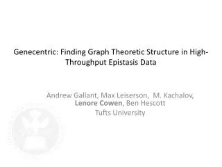
Genecentric: Finding Graph Theoretic Structure in High-Throughput Epistasis Data . Andrew Gallant, Max Leiserson , M. Kachalov , Lenore Cowen , Ben Hescott Tufts University . Protein-protein interaction. High-throughput Interaction Data: aka ‘The Hairball’. What we want:. What we have:.

Genecentric: Finding Graph Theoretic Structure in High-Throughput Epistasis Data
E N D
Presentation Transcript
Genecentric: Finding Graph Theoretic Structure in High-Throughput Epistasis Data Andrew Gallant, Max Leiserson, M. Kachalov, Lenore Cowen, Ben Hescott Tufts University
What we want: What we have: Question: Can we infer anything about "real" pathways from the low-resolution graph model of pairwise interactions?
The hairball: A simple graph model vertices ↔ genes/proteins edges ↔ physical interactions or genetic interactions • simplifications: • undirected • loses temporal information • difficult to decompose into separate processes • conflates different PPI types into one class of "physical interactions"
Interaction types • We distinguish here between two types of interaction: • physical interactions • genetic interactions
Genetic interactions (epistasis) Only 18% of yeast genes are essential (the yeast dies when they’re removed). For the rest, we can compare the growth of the double knockout to its component single knockouts.
Genetic interactions (epistasis) • For non-essential genes, we can compare the growth of the double knockout to its component single knockouts Picture: Ulitsky
Nonessential Genes • Some genes are non-essential because they are only required under certain conditions (i.e. an enzyme to metabolize a particular nutrient). • Other genes are non-essential because the network has some built-in redundancy. • One gene (completely or partially) compensates for the loss of another. • One functional pathway (completely or partially) compensates for the loss of another.
In reality, the data are very incomplete:Between-Pathway Model (BPM)
Kelley and Ideker (2005) and Ulitsky and Shamir (2007) • Goal: detect putative BPMs in yeast interactome • Method: • find densely-connected subsets of the physical protein-protein interaction (PI) network (putative pathways) • check the genetic interaction (GI) network to see if patterns in density of genetic interactions correlate with these putative pathways • check resulting structures for overrepresentation of biological function (gene set enrichment)
Kelley and Ideker (2005) and Ulitsky and Shamir (2007) (1) (2) enriched for function X enriched for function Y (3)
Kelley and Ideker (2005) and Ulitsky and Shamir (2007) • Problems: • Sparse data limits the potential scope of discovery • independent validation is difficult
Further work on this problem: Synthetic lethality: • Ulitsky and Shamir (2007) • Ma, Tarrone and Li (2008) • Brady, Maxwell, Daniels and Cowen (2009) • Hescott, Leiserson, Cowen and Slonim (2010) Epistasis (weighted) data: -- Kelley and Kingsford (2011) -- Leiserson, Tatar, Cowen and Hescott (2011)
So: what is the right way to generalize BPMs to edge weights?
Quantitative interaction data New methods generates high-throughput data for genetic interactions. -7.3556 -0.6347 E-MAP, Epistatic Miniarray Profile Data is scalar (-22 to 15) Synthetic Lethal, < -2.5 Synthetic Sick, -2.5 < x < 0 Synthetic Rescue, >+2.5 Allevating 0<x< 2.5 SGA, Synthetic Genetic Array (smaller weights, -1.1 to 0.8) 3.69893 3.2723 -5.2571 -1.3668 -3.3368 -5.5312 0.5838 -6.3511
Want most negative weight across -7.32156 3.23673 3.6539866 -7.32156 3.23723 -5.252571 -1.366879 -3.365368 3.68398 -3.36536 -0.66434 -5.506312 0.553838 -5.25271 -5.506312 2.73 -6.315511 0.53838 -1.36879 -6.31511
What is the Quality of a BPM? -7.321556 3.685398 -3.365368 -0.664347 3.236723 -5.252571 2.13473 0.13342 0.553838 -1.366879 -6.315511 Once we obtain a candidate BPM we can score it using interaction data. Sum interactions within Sum interactions between Take the difference and normalize to create an interaction score
Genecentric takes the perspective of each gene in turn -7.321556 3.685398 -3.365368 -0.664347 3.236723 -5.252571 2.13473 0.13342 0.553838 -1.366879 -6.315511 What is the ‘best’ candidate BPM that contains node g? Consider a diverse set of GLOBAL partitions that try to MAXIMIZE our objective function over the whole graph. Which genes are consistently placed in the same (opposite) partition as g?
So we can extract a gene’s best BPM from a diverse set of good global bipartitions Idea for constructing the global bipartitions: Maximal cut
Create a random bipartition For every vertex (gene) assign to a partition at random
Local search method Now for each gene, v, consider its interaction scores
Flip Flip to the other side to make it happy! same(v) is now opposite(v) and opposite(v) is same(v) some vertices could change to happy or unhappy
Important properties Flip will always terminate - finite number of possible partitions - weight between partitions decreases with each flip - everyone is happy eventually - local optimum
How we make a BPM from bipartitions -7.3215 3.6398 -3.3653 -0.66434 3.23672 -5.252571 2.1373 0.13342 0.55338 -1.36679 -6.3151 For every gene run weighted flip on the entire graph of interactions, M times (250 times) Some genes will stay on same side for most runs. Some genes will stay on the opposite side for most runs. Most will switch sides among the different runs
BPM collection: Removing Redundancies -7.321556 Remove BPMs that are too large or small 3.685398 -3.365368 -0.664347 3.236723 -5.252571 Take the difference and divide by the size 2.13473 Sort by score, add to final output set if Jaccard index < .66 for all previously added BPMs 0.13342 0.553838 -1.366879 -6.315511 Numbers chosen to match previous studies
How do we measure results? • FuncAssociate to measure gene set enrichment Berriz, Beaver, Cenik, Tasan, Roth, “Next generation software for functional trend analysis,” Bioinformatics, 2009, 25(22): 3043-4. Location of physical interactions
How does Gencentric work with various data? -7.3215 SGA -0.66434 E-MAP (Cell Cycle) -0.91511 -0.22314 3.6853 3.26723 0.54278 -0.687991 -5.252571 -1.366879 -3.365368 0.983123 0.253228 -5.506312 0.5538 0.404421 -6.315511 -6.31511 -7.22314 -3.12363 -1.687991 -6.63178 -5.7225 -0.22565 -0.55672 -2.404421 E-MAP (s. pombe) 1.2833 -3.355371 4.51368 0.253228 E-MAP (MAP-K) 5.22163 1.23711 -7.137271
Consider physical interactions -7.3215 -0.66434 3.6853 3.236723 -5.252571 -1.366879 -3.365368 -5.506312 0.5538 -7.3556 -6.31511 Physical Interactions 3.5398 -3.33368 -0.66347 genetic interactions 3.2723 -5.25371 2.13473 0.55838 -1.3689 -6.3111
Modifying the weights -7.321556 -0.664347 How does alleviating interaction data affect the results? 3.685398 3.236723 Does a continuum of possible weights change the results? -5.252571 -1.366879 -3.365368 -5.506312 0.553838 Do extreme weights affect the quality of the results? -6.315511
Genecentric: try this at home • Project name: Genecentric • Project homepage: http://bcb.cs.tufts.edu/genecentric • Operating system: platform independent • Programming language: Python • Other requirements: Python 2.6 or higher • License: GNU Public License (GPL 2.0)
Gencentric parameters • Set M (number of randomized bipartitions) default 250 • Set C (consistency of same side/opposite side for inclusion in g’s BPM) default 90% • Set J (Jaccard index, how much overlap before similar BPMs are pruned) default .66 • Do you want a min or max size module? (default 3-25) • FuncAssociate parameters: genespace, p-value
Genecentric works out of the box • “New” E-MAP of plasma membrane genes from Aguilar et al. in 2010. • 374 genes including those known to be involved in endocytosis, signaling, lipid metabolism, eisome function. • Genecentric was run with default E-MAP parameters, except C was lowered from .9 to .8 to produce more BPMs (22 instead of 6)
Genecentric on plasma membrane E-MAP : example BPM BPM1 BPM2 ARL1 VPS35 GET3 ARL3 SYS1 GOT1 PEP8 SFT2 MNN1 VPS17 Protein transport, Golgi apparatus, endsome transport, vesicle-mediated transport • COG6 COG5 COG8 PIB2 COG7 • Intra-Golgi vesicle-mediated transport, protein targeting to vacuole
Genecentric on plasma membrane E-MAP : example BPM BPM1 BPM2 PEX1 PEX6 EDE1 SKN7 ERG4 ADH1 PEX15 ARC18 EMC33 Protein import into peroxisome matrix, receptor recycling • SLT2 BCK1 CLC1 • Endoplasmic reticulum unfolded protein response
Biological Findings (cont.) • Some complexes come up again and again– could they be global mechanisms of fault tolerance? In Plasma Membrane; -- COG complex In Chrombio; • SWR-C complex (Chromatin remodeling) • Prefoldin complex (Chaperone) • MRE11 complex (DNA damage repair)
Co-authors and collaborators • Ben Hescott • Max Leiserson • Diana Tartar • Maxim Kachalov
A Graph Theory Problem Our algorithm samples from the maximal bipartite subgraphs. With what distribution? Is it uniform? Proportional to the number of edges that cross the cut?? ??? What are the properties of the stable bipartite subgraphs of the synthetic lethal network? Are they conserved across species?
Approach • Run the partitioning algorithm 250 times on the yeast SL network (G). • For each gene g in G, • Construct a set A consisting of g and all nodes in G which wind up in the same set as g at least 70% of the time. • Construct another set B consisting of all nodes in G which wind up in the opposite set from g at least 70% of the time. • We call the subgraph of G defined by A and B the “stable bipartite subgraph of g”, and designate it as a candidate BPM.
Delete a gene in pathway 1; see if changes in pathway 2 coherent