Simulating Coin Tosses to Estimate the Expected Value of Gap(N)
This document outlines a method to simulate a game of tossing a fair coin until the absolute difference between the counts of Heads and Tails reaches a specified number N. It includes a function, Gap(N), to return the total tosses required. It also demonstrates how to compute the average score over multiple games, allowing for the estimation of the expected value of Gap(N). Sample outputs for various values of N are provided to illustrate the method's effectiveness, showcasing how expected values converge as the number of trials increases.

Simulating Coin Tosses to Estimate the Expected Value of Gap(N)
E N D
Presentation Transcript
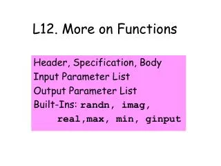
L12. More on Functions Header, Specification, Body Input Parameter List Output Parameter List Built-Ins: randn, imag, real,max, min, ginput
Eg. 1: “Gap N” Keep tossing a fair coin until | Heads – Tails | == N Score = total # tosses Write a function Gap(N) that returns the score and estimate the average value.
The Packaging… function nTosses = Gap(N) Heads = 0; Tails = 0; nTosses = 0; while abs(Heads-Tails) < N nTosses = nTosses + 1; if rand <.5 Heads = Heads + 1; else Tails = Tails + 1; end end
The Header… function nTosses = Gap(N) output parameter list input parameter list
The Body Heads = 0; Tails = 0; nTosses = 0; while abs(Heads-Tails) < N nTosses = nTosses + 1; if rand <.5 Heads = Heads + 1; else Tails = Tails + 1; end end The necessary output value is computed.
Local Variables Heads = 0; Tails = 0; nTosses = 0; while abs(Heads-Tails) < N nTosses = nTosses + 1; if rand <.5 Heads = Heads + 1; else Tails = Tails + 1; end end
A Helpful Style Heads = 0; Tails = 0; n = 0; while abs(Heads-Tails) < N n = n + 1; if rand <.5 Heads = Heads + 1; else Tails = Tails + 1; end end nTosses = n; Explicitly assign output value at the end.
The Specification… function nTosses = Gap(N) % Simulates a game where you % keep tossing a fair coin % until |Heads - Tails| == N. % N is a positive integer and % nTosses is the number of % tosses needed.
Estimate Expected Valueof Gap(N) Strategy: Play “Gap N” a large number of times. Compute the average “score.” That estimates the expected value.
Solution… N = input('Enter N:'); nGames = 10000; s = 0; for k=1:nGames s = s + Gap(N); end ave = s/nGames; A very common methodology for the estimation of expected value.
Sample Outputs N = 10 Expected Value = 98.67 N = 20 Expected Value = 395.64 N = 30 Expected Value = 889.11
Solution… N = input('Enter N:'); nGames = 10000; s = 0; for k=1:nGames s = s + Gap(N); end ave = s/nGames; Program development is made easier by having a function that handles a single game.
What if the Game WasNot “ Packaged”? s = 0; for k=1:nGames score = Gap(N) s = s + score; end ave = s/nGames;
Heads = 0; Tails = 0; nTosses = 0; while abs(Heads-Tails) < N nTosses = nTosses + 1; if rand <.5 Heads = Heads + 1; else Tails = Tails + 1; end end score = nTosses; s = 0; for k=1:nGames score = Gap(N) s = s + score; end ave = s/nGames; A more cumbersome implementation
Is there a Pattern? N = 10 Expected Value = 98.67 N = 20 Expected Value = 395.64 N = 30 Expected Value = 889.11
New Problem Estimate expected value of Gap(N) for a range of N-values, say, N = 1:30
Pseudocode for N=1:30 Estimate expected value of Gap(N) Display the estimate. end
Pseudocode for N=1:30 Estimate expected value of Gap(N) Display the estimate. end Refine this!
Done that.. nGames = 10000; s = 0; for k=1:nGames s = s + Gap(N); end ave = s/nGames;
Sol’n Involves a Nested Loop for N = 1:30 % Estimate the expected value of Gap(N) s = 0; for k=1:nGames s = s + Gap(N); end ave = s/nGames; disp(sprintf('%3d %16.3f',N,ave)) end
Sol’n Involves a Nested Loop for N = 1:30 % Estimate the expected value of Gap(N) s = 0; for k=1:nGames s = s + Gap(N); end ave = s/nGames; disp(sprintf('%3d %16.3f',N,ave)) end But during derivation, we never had to reason about more than one loop.
Output N Expected Value of Gap(N) -------------------------------- 1 1.000 2 4.009 3 8.985 4 16.094 28 775.710 29 838.537 30 885.672 Looks like N2. Maybe increase nTrials to solidify conjecture.
Eg. 2: Random Quadratics Generate random quadratic q(x) = ax2 + bx + c If it has real roots, then plot q(x) and highlight the roots.
Built-In Function: randn % Uniform for k=1:1000 x = rand; end % Normal for k=1:1000 x = randn; end
Built-In Functions: imag and real x = 3 + 4*sqrt(-1); y = real(x) z = imag(x) Assigns 3 to y. Assigns 4 to z.
Built-In Functions: min and max a = 3, b = 4; y = min(a,b) z = max(a,b) Assigns 3 to y. Assigns 4 to z.
Packaging the CoefficientComputation function [a,b,c] = randomQuadratic % a, b, and c are random numbers, % normally distributed. a = randn; b = randn; c = randn;
Input & Output Parameters function [a,b,c] = randomQuadratic A function can have no input parameters. Syntax: Nothing A function can have more than one output parameter. Syntax: [v1,v2,… ]
Computing the Roots function [r1,r2] = rootsQuadratic(a,b,c) % a, b, and c are real. % r1 and r2 are roots of % ax^2 + bx +c = 0. r1 = (-b - sqrt(b^2 - 4*a*c))/(2*a); r2 = (-b + sqrt(b^2 - 4*a*c))/(2*a);
Question Time function [r1,r2] = rootsQuadratic(a,b,c) r1 = (-b - sqrt(b^2 - 4*a*c))/(2*a); r2 = (-b + sqrt(b^2 - 4*a*c))/(2*a); a = 4; b = 0; c = -1; [r2,r1] = rootsQuadratic(c,b,a); r1 = r1 Output? A. 2 B. -2 C. .5 D. -.5
Answer is B. We are asking rootsQuadratic to solve -x2 + 4 = 0 roots = +2 and -2 Since the function ca ll is equivalent to [r2,r1] = rootsQuadratic(-1,0,4); Script variable r1 is assigned the value that rootsQuadratic returns through output parameter r2.That value is -2
Script Pseudocode for k = 1:10 Generate a random quadratic Compute its roots If the roots are real then plot the quadratic and show roots end
Script Pseudocode for k = 1:10 Generate a random quadratic Compute its roots If the roots are real then plot the quadratic and show roots end [a,b,c] = randomQuadratic;
Script Pseudocode for k = 1:10 [a,b,c] = randomQuadratic; Compute its roots If the roots are real then plot the quadratic and show roots end [r1,r2] = rootsQuadratic(a,b,c);
Script Pseudocode for k = 1:10 [a,b,c] = randomQuadratic; [r1,r2] = rootsQuadratic(a,b,c); If the roots are real then plot the quadratic and show roots end if imag(r1)==0 && imag(r2)===0
Script Pseudocode for k = 1:10 [a,b,c] = randomQuadratic; [r1,r2] = rootsQuadratic(a,b,c); if imag(r1)==0 && imag(r2)==0 then plot the quadratic and show roots end end
Plot the Quadraticand Show the Roots m = min(r1,r2); M = max(r1,r2); x = linspace(m-1,M+1,100); y = a*x.^2 + b*x + c; plot(x,y,x,0*y,':k',r1,0,'or',r2,0,'or')
Plot the Quadraticand Show the Roots m = min(r1,r2); M = max(r1,r2); x = linspace(m-1,M+1,100); y = a*x.^2 + b*x + c; plot(x,y,x,0*y,':k',r1,0,'or',r2,0,'or') This determines a nice range of x-values.
Plot the Quadraticand Show the Roots m = min(r1,r2); M = max(r1,r2); x = linspace(m-1,M+1,100); y = a*x.^2 + b*x + c; plot(x,y,x,0*y,':k',r1,0,'or',r2,0,'or') Array ops get the y-values.
Plot the Quadraticand Show the Roots m = min(r1,r2); M = max(r1,r2); x = linspace(m-1,M+1,100); y = a*x.^2 + b*x + c; plot(x,y,x,0*y,':k',r1,0,'or',r2,0,'or') Graphs the quadratic.
Plot the Quadraticand Show the Roots m = min(r1,r2); M = max(r1,r2); x = linspace(m-1,M+1,100); y = a*x.^2 + b*x + c; plot(x,y,x,0*y,':k',r1,0,'or',r2,0,'or') A black, dashed line x-axis.
Plot the Quadraticand Show the Roots m = min(r1,r2); M = max(r1,r2); x = linspace(m-1,M+1,100); y = a*x.^2 + b*x + c; plot(x,y,x,0*y,':k',r1,0,'or',r2,0,'or') Highlight the root r1 with red circle.
Plot the Quadraticand Show the Roots m = min(r1,r2); M = max(r1,r2); x = linspace(m-1,M+1,100); y = a*x.^2 + b*x + c; plot(x,y,x,0*y,':k',r1,0,'or',r2,0,'or') Highlight the root r2 with red circle.
Complete Solution for k=1:10 [a,b,c] = randomQuadratic; [r1,r2] = rootsQuadratic(a,b,c); if imag(r1)==0 m = min(r1,r2); M = max(r1,r2); x = linspace(m-1,M+1,100); y = a*x.^2 + b*x + c; plot(x,y,x,0*y,':k',r1,0,'or',r2,0,'or') shg pause(1) end end