Download
1 / 110
1.11k likes | 1.58k Vues
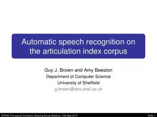
Sequence Scoring Experiments Using the TIMIT Corpus and the HTK Recognition Framework. Author : Arthur Gerald Kunkle Committee Chair : Dr. Veton Z. Këpuska. ASR Defined. Automatic Speech Recognition (ASR) - mapping an acoustic signal into a string of words.

E N D
Sequence Scoring Experiments Using the TIMIT Corpus and the HTK Recognition Framework Author: Arthur Gerald Kunkle Committee Chair: Dr. Veton Z. Këpuska
ASR Defined • Automatic Speech Recognition (ASR) - mapping an acoustic signal into a string of words. • ASR systems play a big role in Human Machine Interaction (HMI). • Speech has a natural potential to be much more intuitive to use to command a machine versus the existing input methods, such as keyboard and mouse.
Early ASR Systems • Earliest systems for ASR would model natural resonances that occur as a result of air flowing over the vocal tract creating sounds • Example: To recognize the digit “five”, the system would determine that the vowel sound “eye” matched the correct digit. • Limitation - Utterance contained only a single digit and no other word or non-speech event that would confuse the system.
ASR Improvements • ASR System Development in the 1980s and 1990s introduced use of Hidden Markov Models (HMMs). • Still widely used over the past two decades • Improvements being made on a continual basis. • ASR received interest from DARPA, leading to new and notable ASR systems such as the CMU Sphinx (Carnegie Mellon University) system. • Formalized the tasks and evaluation criterion that were used to measure ASR System Performance.
Characteristics of ASR Systems • ASR Systems are defined by the tasks they are designed to solve. • We have already discussed some examples of tasks. • Tasks involve the following parameters: • Vocalbulary Size • Fluency • Environmental Effects • Speaker Characteristics
Vocabulary Size • Milestones in ASR Systems are often related to how large of a vocabulary a system can handle while keeping error rate at a minimum. • Simple Task Vocabulary: Recognizing digits: • “zero,” “one,” “two,”…, and “oh” • These eleven words are the in-vocabulary words (INV). • If the system encounters any words outside of this set, they are known as out-of-vocabulary words (OOV).
ASR Tasks and Vocabulary Sizes • As vocabulary size of a task increases, so does the Word Error Rate (WER). • WER is the standard evaluation metric for speech recognition
Example WER Calculation • This example is an output hypothesis of a string of numbers from an ASR system, compared with the true sentence string. The bottom line marks the types of errors as they occur in the transcription.
ASR System Fluency • Fluency measures the rigidity of input speech. • In isolated-wordrecognition, the speech to be processed is surrounded by a known silence or pause. • Examples include the digit recognition or command-and-control tasks. • Continuous-speech systems must take non-speech events and segmentation of real words into account. • This is much harder to accomplish!
Other ASR System Parameters • Environmental noise and channel characteristics. • Recording instruments may be located at different distances from each speaker and may pick up other noises in addition to speech. • Speaker-dependant characteristics. • Speaker dialect and accent.
Wake-up-Word Paradigm • The Wake-up-Word (WUW) ASR Problem: • Detect a single word or phrase when spoken in an alerting context, while rejecting all other words, phrases, sounds, noises and other acoustic events with virtually 100% accuracy including the same word or phrase of interest spoken in a non-alerting (i.e. referential) context.
WUW Example Application • User utters the WUW “Computer” to alert a machine to perform various commands. • When the user utters the command phrase “Computer, begin presentation,” WUW technology should detect that “Computer” was spoken in the alerting context and perform the requested command. • If the user utters the phrase “I want to buy a new computer,” WUW technology must detect that “Computer” was used in a non-alerting context and avoid parsing the command.
WUW Problem Areas • Detecting WUW Context – The WUW system must be able to notify the host system that attention is required in certain circumstances and with high accuracy. Unlike keyword-spotting ,WUW dictates these occurrences only be reported during an alerting context. This context can be determined using features such as leading and trailing silence, difference in the long term average of speech features, and prosodic information (pitch, intonation, rhythm, etc.). • Identifying WUW – After identifying the correct context for a spoken utterance, the WUW paradigm shall be responsible for determining if the utterance contains the pre-defined Wake-up-Word to be used for command (e.g. “Computer”) with a high degree of accuracy, e.g., > 99%. • Correct Rejection of Non-WUW – Similar to identification of the WUW, the system shall also be capable of filtering speech tokens that are not WUWs with practically 100% accuracy to guarantee 0% false acceptances.
Current WUW System • Currently being used for practical applications such as: PowerPoint Commander, Elevator Simulator, Car Inspection System, and Nursing Call Center
Motivations for External Scoring Toolkit • Support for standard speech recognition testing data sets. Provide support for evaluating the TIMIT data set in order to evaluate novel scoring methods against a broader class of words. • Integration of standard toolkits. Utilizethe Hidden Markov Model Toolkit (HTK) and the SVM library (LIBSVM) to build and evaluate HMM and SVM models. Using industry-standard frameworks has the benefit of a well-documented environment and previous results. • Integration of novel scoring techniques with standard toolkits. The novel method used in the WUW system must be integrated with the existing workflow in the HTK framework in order to augment the technique and evaluate its effectiveness against additional data sources. • Provide MATLAB-based analysis and experimentation tools. Once results are obtained using the SeqRec tools for HTK and LIBSVM, MATLAB scripts will be used to provide visualization of the results. • Provide support for One-Class SVM modeling. A technique that allows a recognition model to be built on only INV data scores. This SVM type will be applied to WUW and the benefits and disadvantages will be explored.
SeqRec System Overview • In order to further explore and refine the unique speech recognition elements of the WUW system, the Sequence Recognizer (SeqRec) Toolkit was developed.
Speech Recognition Goals • Speech recognition systems often assume speech is a realization of some message encoded as a sequence of one or more discrete symbols. • Speech is normally converted into a sequence of equally spaced discrete parameter vectors. (typically every 10ms). • Makes the assumption that a speech waveform can be regarded as a stationary process over the sampling time
Speech Recognition Goals, contd. • The speech recognizer’s job is to create a mapping between the sequences of speech frames and the underlying speech symbols that constitute the utterance.
Probability Theory of ASR • “What is the most likely discrete symbol sequence out of all valid sequences in the language L, given some acoustic input O?” • Acoustic Input is set of discrete observations: • Symbol sequence is defined as: • Fundamental ASR System Goal:
Probability Theory of ASR, contd. • Applying Bayes’ Theorem: • New quantities are easier to compute than P(W |O). • P(W) is defined as the prior probability for the sequence itself. This is calculated by using the prior knowledge of occurrences of the sequence W. • P(O) is the prior probability of the acoustic input occurrence.
Probability Theory of ASR, contd. • P(O) is not needed, because the argmax expression implies we will be calculating over all possible sequences. • The probability P(O|W), which is the likelihood of the acoustic input O, given the sequence W, is defined as the observation likelihood. (often referred to as the acoustic score) • This quantity can be determined using the Hidden Markov Model.
Elements of HMMs • The set of states constituting the model. Although the states themselves are “hidden” from the perspective of state assignment of each observation vector, the exact number of states often carries a physical significance
Elements of HMMs, contd. • The transition probability matrix. Each element of this matrix represents the probability of transitioning from state i to state j. Each row of this matrix must sum to 1 to be valid.
Elements of HMMs, contd. • The emission probabilities. Each of these expresses the probability of an observation being generated during state i. Note that the beginning and end states of an HMM do not have an associated emission probability.
Elements of HMMs, contd. • The probability distribution of starting in each state.
Elements of HMMs, contd. • The following equation is used to express all the parameters of an HMM in a compact form:
ASR HMMs • An ASR HMM is normally used to model a phoneme. • Smallest distinguishable sound unit in a language. • Generally have three emitting states in order to model the transition-in, steady state, and transition-out regions of the phoneme. • Whole word HMM is created by simply concatenating the phonemes used to spell the word in question.
Acoustic Scores Using HMMs • So how do we use HMMs to calculate the probability of an observation sequence, given a specific model? • Restated: Score how well a given model matches an input observation sequence. • For HMMs, each hidden state produces only a single observation. • Length(sequence of traversed states) == Length(sequence of observation)
Acoustic Scores Using HMMs, contd. • The actual state sequence that observation sequence will take is hidden. • Assuming independence, have to calculate joint probability of a particular observation sequence and a particular state sequence: • This probability must be calculated across all valid state sequences in the model:
Acoustic Scores Using HMMs, contd. • While this solution is valid, it presents a calculation that requires O(N^T) computations. • For speech processing applications of HMM, these parameters can become quite large. • In order to reduce the amount of calculations needed, the forward algorithm is used.
Forward Algorithm • The forward algorithm is a dynamic programming technique that uses a table to store intermediate values as it builds the final probability of the observation sequence. • Each cell is calculated by summing over the extensions in all paths that lead to the current cell.
Forward Algorithm, contd. • The forward algorithm is a three step process: • Initialization: • Induction: • Termination:
HMM Paramter Re-estimation • HMM parameter re-estimation is how we should adjust the model parameters in order to maximize the acoustic score. • This problem is addressed by using the Baum-Welch algorithm.
HMM Paramter Re-estimation, contd. • Goal for Re-estimating the transition probability matrix A: • Goal for Re-estimating the emission probability distributions:
HMM Paramter Re-estimation, contd. • These calculations lead to the following equations. (See Rabiner for details and derivations.)
HMM Paramter Re-estimation, contd. • If a current model is re-estimated using the EM algorithm to create a new, refined model, then either: • The initial model defines a critical point of the likelihood function, in which case (no HMM parameter updates were made). • A new model has been discovered that describes an HMM in which an observation sequence O is more likely to have been produced. • The final model produced by EM is called the maximum likelihood HMM.
Speech-Specific HMM Recognition • The previous section presented the fundamentals associated with using HMMs to perform general sequence recognition. • There are some additional concepts associated specifically with the speech recognition task domain: • Feature Representation of Speech • Gaussian Mixture Model Distributions
Feature Representation of Acoustic Speech Signals • The input to an ASR system is normally a continuous speech waveform. • This input must be transformed into a sequence of acoustic feature vectors, each of which captures a small amount of information within the original waveform.
Feature Representation of Acoustic Speech Signals, contd. • Pre-emphasis – This stage is used to amplify energy in the high-frequencies of the input speech signal. This allows information in these regions to be more recognizable during HMM model training and recognition.
Feature Representation of Acoustic Speech Signals, contd. • Windowing – This stage slices the input signal into discrete time segments. A Hamming window is commonly used to prevent edge effects associated with the sharp changes in a Rectangular window.
Feature Representation of Acoustic Speech Signals, contd. • Discrete Fourier Transform – DFT is applied to the windowed speech signal, resulting in the magnitude and phase representation of the signal.
Feature Representation of Acoustic Speech Signals, contd. • Mel Filter Bank - Human hearing is less sensitive at frequencies above 1000 Hz. so the spectrum is warped using a logarithmic Mel scale. A bank of filters is constructed with filters distributed equally below 1000 Hz and spaced logarithmically above 1000 Hz
Feature Representation of Acoustic Speech Signals, contd. • Inverse DFT – The IDFT of the Mel spectrum is computed, resulting in the cepstrum. This representation is valuable because it separates characteristics of the source and filter of the speech waveform. The first 12 values of the resulting cepstrum are recorded. • Delta MFCC Features – In order to capture the changes in speech from frame-to-frame, the first and second derivative of the MFCC coefficients are also calculated and included.
Feature Representation of Acoustic Speech Signals, contd. • Energy Feature – This step is performed in parallel with the MFCC feature extraction and involves calculating the total energy of the input frame.
Feature Representation of Acoustic Speech Signals, contd. • Results in a 39-element Observation Vector for each Frame of Speech
Gaussian Mixture Models • Until now, the emission probability associated with an HMM state was left as a general probability distribution. • In most ASR systems, these output probabilities are continuous-density multivariate output distributions. • The most common form of this distribution used in speech recognition is the Gaussian Mixture Model (GMM).
Gaussian Mixture Models, contd. • A simple Gaussian distribution describing a one-dimensional random variable X is described by the mean and variance