Improving the Chlorophyll Algorithm
Improving the Chlorophyll Algorithm. Janet W. Campbell University of New Hampshire Ocean Color Science Team Meeting Newport, RI April 12, 2006. Why? Isn’t it time to get on with the science … beyond chlorophyll?. Yes .. It is time to get beyond chlorophyll.

Improving the Chlorophyll Algorithm
E N D
Presentation Transcript
Improving the Chlorophyll Algorithm Janet W. Campbell University of New Hampshire Ocean Color Science Team Meeting Newport, RI April 12, 2006
Why? Isn’t it time to get on with the science … beyond chlorophyll? Yes .. It is time to get beyond chlorophyll. However, if there is to be one climate data record produced from ocean color satellite data, it is mostly likely to be chlorophyll. Thus, we should do everything we can to ensure that there is continuity in the chlorophyll time series from SeaWiFS to MODIS to NPP to VIIRS.
MODIS is currently producing the “SeaWiFS-analog” chlorophyll product based on the OC3M algorithm. SeaWiFS uses the OC4.v4 algorithm. Both algorithms were parameterized with the same data set used (n = 2,804). OC3M Both are described in NASA TM 2000-206892, Vol. 11 (O’Reilly et al., 2000).
but the algorithms are different… The algorithms are similar… The SeaWiFS algorithm (OC4.v4) is: log10(CHL) =0.366 – 3.067R + 1.930R2 + 0.649R3 – 1.532R4 where R = log10[max(Rrs(443), Rrs(490), Rrs(510))/ Rrs(555)] The MODIS algorithm (OC3M) is: log10(CHL) = 0.283 – 2.753R + 1.457R2 + 0.659R3 – 1.403R4 where R = log10[max(Rrs(443), Rrs(488))/ Rrs(551)]
There are systematic differences between the OC3M and OC4 algorithms even when applied to the same data set (assuming 488 ~ 490, 551 ~ 555)
RECOMMENDATIONS (April 2005) • The MODIS and SeaWiFS chlorophyll algorithms should be mutually consistent to allow the creation of a climate data record (1997-present). • Use newly created in situ data set (NOMAD) to test candidate algorithms. I proposed to host another “SeaBAM” workshop at UNH to evaluate candidate algorithms. • As a minimum, we should aim to develop an algorithm that can solve for CDOM and Chl-a simulaneously.
OUTLINE: TODAY’S TALK • Resolving differences between SeaWiFS and MODIS algorithms • Ocean Color Bio-optical Algorithm Mini (OCBAM) Workshop – Sept. 2005 • Goals, motivation, and groundrules • Conclusions / recommendations / followup • Quantifying the performance / uncertainty of the chlorophyll algorithm(s) • Systematic trends in errors discovered!
Resolving differences between SeaWiFS and MODIS algorithms The assumption that Rrs(551) ~ Rrs(555) is wrong! (Thanks to Jeremy Werdell for figuring this out!)
OUTLINE: TODAY’S TALK • Resolving differences between SeaWiFS and MODIS algorithms • Ocean Color Bio-optical Algorithm Mini (OCBAM) Workshop – Sept. 2005 • Goals, motivation, and groundrules • Conclusions / recommendations / followup • Quantifying the performance / uncertainty of the chlorophyll algorithm(s) • Systematic trends in errors discovered! √
Ocean Color Bio-optical Algorithm Mini (OCBAM) Workshop University of New Hampshire Durham, New Hampshire September 27-29, 2005
Attendees: Dirk Aurin University of Connecticut Sean Bailey NASA Goddard Space Flight Center Shane Bradt University of New Hampshire Paula Bontempi NASA Headquarters Janet Campbell Ocean Process Analysis Lab, UNH Mark Dowell Joint Research Center, Ispra, Italy Robert Frouin University of California - San Diego Carol Fairfield NMFS Visiting Scientist, UNH Hui Feng Ocean Process Analysis Lab, UNH Paul Lyons ORBIMAGE, Inc. Haymarket, VA Chuck McClain NASA Goddard Space Flight Center Stephane Maritorena University of California - Santa Barbara Timothy Moore Ocean Process Analysis Lab, UNH Ru Morrison Ocean Process Analysis Lab, UNH Jay O'Reilly NMFS Narragansett Laboratory Heidi Sosik Woods Hole Oceanographic Institution Chuck Trees San Diego State University Jeremy Werdell NASA Goddard Space Flight Center
Goals The OCBAM workshop was aimed at evaluating ocean color algorithms that produce chlorophyll retrievals. Algorithms tested may also retrieve other constituents and / or related inherent optical properties. Our goal was (still is) to determine how new algorithms perform compared to the operational empirical algorithms (OC4, OC3M) and to evaluate whether improved accuracy is achieved by accounting for other optically active constituents.
Motivation • NOMAD. We have a new data set to use in evaluating algorithms. Werdell, P.J. and S.W. Bailey, 2005: An improved bio-optical data set for ocean color algorithm development and satellite data product validation. Remote Sensing of Environment , 98(1), 122-140.
Motivation • NOMAD. We have a new data set to use in evaluating algorithms. • Concern that the operational algorithms used for SeaWiFS (OC4) and MODIS (OC3M) be mutually consistent.
Motivation • NOMAD. We have a new data set to use in evaluating algorithms. • Concern that the operational algorithms used for SeaWiFS (OC4) and MODIS (OC3M) be mutually consistent. • A recent paper in (Siegel et al. 2005) argues for the importance of accounting for the effects of colored dissolved organic matter.
A paper entitled “Colored dissolved organic matter and its influence on the satellite-based characterization of the ocean biosphere” by D. Siegel, S. Maritorena, N. Nelson, M. Behrenfeld, and C. McClain has appeared Geophysical Research Letters. The authors applied the GSM01 algorithm to global SeaWiFS data and compared the derived chlorophyll distributions with OC4 chlorophyll maps. Differences are quite significant – and this paper will predictably cause a stir. We should be prepared to respond …
OCBAM Groundrules (Rules of Engagement) Any algorithm approach may be considered. This is not a workshop to look only at “semi-analytical” algorithms. Algorithms will be evaluated using a common data set (a subset of NOMAD) and common performance criteria. We should regard the OC4 and OC3M as the “algorithms to beat.” Compare your results with these operational algorithms, not with other non-operational ones.
If we can resolve other optical properties or constituents (e.g., CDOM, POC) all the better … but our focus should remain on chlorophyll. The challenge is to explain and reduce the errors in Chl with an algorithm that can be implemented practically. Issues related to its practical application include its speed, sensitivity to errors in Lwn, and ability to converge on a solution.
Conclusions / recommendations from the workshop… Very little improvement in the chlorophyll algorithm can be achieved without accounting for the effects of other optically active constituents. It is time to start pushing the envelop toward algorithms that yield information about dissolved and particulate materials as well as the chlorophyll concentration. It is generally believed that this will require model-based (“semi-analytic”) algorithms instead of the empirical algorithms such as OC4 and OC3M.
Conclusions / recommendations from the workshop… The Ocean Biology Data Processing Group at NASA Goddard is prepared to run algorithm codes and produce metrics for anyone wishing to have an algorithm considered as a candidate for the next generation of ocean color algorithms. Our goal is to arrive at a consensus algorithm based on commonly agreed upon performance metrics.
The Ocean Biology Data Processing Group at Goddard (GBDPG) has set up a website that has the powerpoint presentations from the workshop, several relevant documents, and results of post-workshop analyses. http://oceancolor.gsfc.nasa.gov/MEETINGS/OCBAM/This site is password protected. The password is the same as that used to access SeaWiFS data from the OceanColor online browse pages. A full description of the metrics to be used in comparing algorithms has been posted on the website -- look for document entitled "Performance Metrics."
Anyone who has an algorithm to propose is welcome to participate. We ask that you use the NOMAD subset which is posted on the OCBAM website. Please submit your retrievals (chlorophyll and other properties e.g., acdm, bbp, etc.) to the ftp site (next page) in a table or spreadsheet which includes, as a minimum, the index identifying the station. We also ask that you submit a copy of your code so that it can be run by the OBDPG.
The FTP site can be accessed either with command lines or via a browser as follows:* for those using command line FTP access:ftp://samoa.gsfc.nasa.govuser: ocbampass: inversion* for those using a Web browser:ftp://ocbam:inversion@samoa.gsfc.nasa.gov(the only difference being where one types in the username and password)Here you will be able to upload your results and codes for evaluation by the OBDPG.
OUTLINE: TODAY’S TALK • Resolving differences between SeaWiFS and MODIS algorithms • Ocean Color Bio-optical Algorithm Mini (OCBAM) Workshop – Sept. 2005 • Goals, motivation, and groundrules • Conclusions / recommendations / followup • Quantifying the performance / uncertainty of the chlorophyll algorithm(s) • Systematic trends in errors discovered! √ √
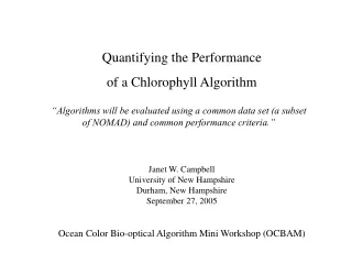
Metrics for Quantifying the Uncertainty in a Chlorophyll Algorithm: Explicit equations and examples using the OC4.v4 algorithm and NOMAD Janet W. Campbell & John E. O’Reilly January 3, 2006 Summary This document describes statistical procedures for quantifying the uncertainty associated with a single retrieval of a chlorophyll algorithm using a data base of coincident optical properties and chlorophyll-a concentration measured in situ. The procedures are actually more general than just chlorophyll and would apply to any property that varies over several orders of magnitude. Explicit equations are given, and the method is demonstrated by quantifying the uncertainty of the SeaWiFS chlorophyll algorithm, OC4.v4, using the newly published NASA bio-Optical Marine Algorithm Data set (NOMAD). …. . . .
Error Definitions The zero-th order definition of error is the log-error: d = The OC4/OC3M polynomials minimize the mean square d:
Error Definitions Log error: d = = Relative error: relerr = = or percentage error = relerr * 100% is often desired. The log error and relative error are directly related: d =
For every point in NOMAD, you can calculate di and relerri (i = 1,…,N). di
Characterize the distribution of log errors in terms of their mean, standard deviation, and root-mean-square. The histogram of di … is symmetric and ~ normally distributed.
The log errors are difficult to interpret because they are in log units (decades). The histogram can easily be converted to a more meaningful one by labeling the axis in terms of the ratio . Note that the scale hasn’t changed – only the labels. If log( ) is normally distributed, then is lognormally distributed.
Statistics of relerr can be derived from the data (empirically) or, if the di errors are normally distributed, relerr statistics can be derived from the log error statistics (see Performance Metrics).
The performance measures derived from NOMAD or any database are influenced by the distribution of the stations in the database. Often there’s an over abundance of high chlorophyll stations. Distribution of chlorophyll in the SeaWiFS climatology (1997-2005) (red) compared with that in NOMAD (blue). Chlorophyll, mg m-3
Log errors (di) for OC4.v4 vs. measured chlorophyll. The red curve is the SeaWiFS distribution shown on the previous slide.
One way to adjust for differences in the distributions of the data (vs. real world) is to bin the data and characterize errors within bins. Then weight the statistics according to the frequency of the global real-world distribution.
SeaWiFS Climatological Chlorophyll (1997-2005) 100 10 1 0.1 0.01
Uncertainty (RMSE) Mapped to SeaWiFS Climatology 0.55 0.50 0.45 0.40 0.35 0.30 0.25 0.20 0.15 Note: This RMSE reflects the uncertainty in a single retrieval. The true uncertainty for this climatology should consider variance reduction due to averaging out random errors. Question: what errors are truly random?
3-band SeaWiFS algorithm: OC3S v5
OUTLINE: TODAY’S TALK • Resolving differences between SeaWiFS and MODIS algorithms • Ocean Color Bio-optical Algorithm Mini (OCBAM) Workshop – Sept. 2005 • Goals, motivation, and groundrules • Conclusions / recommendations / followup • Quantifying the performance / uncertainty of the chlorophyll algorithm(s) • Systematic trends in errors discovered! √ √ √
Large portion of the NOMAD data are from Palmer Station. There are define systematic errors associated with these data!