Download
1 / 19
190 likes | 407 Vues
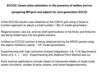
ECCO2: Ocean state estimation in the presence of eddies and ice (preparing MITgcm and adjoint for next-generation ECCO) A first ECCO2 solution was obtained on the CS510 grid using a Green’s function approach to adjust a small number (~80) of model parameters.

E N D
ECCO2: Ocean state estimation in the presence of eddies and ice (preparing MITgcm and adjoint for next-generation ECCO) A first ECCO2 solution was obtained on the CS510 grid using a Green’s function approach to adjust a small number (~80) of model parameters. Regional ocean, sea ice, and ice shelf optimizations in the Arctic and Antarctic are being folded back into the global solution. A follow-on ECCO2 solution is being obtained during the ARGO period using the adjoint method to adjust ~109 model parameters. Experimenting with high-resolution forward integrations (1/8, 1/16-deg forward, Arctic at 9, 4, 2, 1-km). Experimenting with Material Point Method sea ice. Early science applications include impact of mesoscale eddies on large-scale ocean circulation, studies of polar oceans, and ocean biogeochemistry.
Need for high resolution Eddy-parameterizations are not based upon fundamental principles and fail to adequately account for flow anisotropies leading to flux errors that accumulate and change large scale ocean circulation in important ways. Narrow western and eastern boundary currents make major contributions to scalar property transports but are not parameterizable. Until they are resolved, there will be doubts that ocean models carry property transports realistically. Inability to resolve major topographic features (e.g., fracture zones, sills, overflows) leads to systematic errors in movement of deep water masses with consequences for accuracy of water mass formation and properties. Hill et al., 2007
Need for sea ice Sea ice affects radiation balance, surface heat and mass fluxes, ocean convection, freshwater fluxes, human operations, etc. Sea-ice processes impact high-latitude oceanic uptake and storage of anthropogenic CO2 and other greenhouse gases. Inclusion of a dynamic/thermodynamic sea ice model permits fuller utilization of high-latitude satellite data. Kwok et al., 2008
Need for physically consistent assimilation The temporal evolution of data assimilated estimates is physically inconsistent (e.g., budgets do not close) unless the assimilation’s data increments are explicitly ascribed to physical processes (i.e., inverted). Filtered Estimate: x(t+1)=Ax(t)+Gu(t)+(t) x: model state, u: forcing etc, : data increment Data Smoothed Estimate: x(t+1)=Ax(t)+Gu(t) Data increment: time Model Physics: A, G I. Fukumori, JPL
Example: Atmospheric Mass Budget Standard deviation of NCEP surface pressure analysis shows that, on average, 24%of the atmosphere’s mass change is physically unaccounted for (I. Fukumori, JPL). Change over 6-hours Data Increment mbar Atmospheric reanalyses contain huge air-sea flux imbalances. Compare 6.2 cm/yr freshwater flux imbalance to observed 3 mm/yr sea level rise (P. Heimbach, MIT). 1993-2003 global mean air-sea freshwater flux
Example: Sensitivity of CO2 Sea Air Flux Filtered estimate of CO2 flux during 97-98 El Niño (mol/m2/yr) Observed estimate of CO2 flux during 92-93 El Niño Smoothed estimate of CO2 flux McKinley, 2002 Feely et al., 1999
1992-present Green’s function optimization of CS510 MITgcm model configuration • Data constraints: • sea level anomaly • time-mean sea level • - sea surface temperature • temperature and salinity profiles • sea ice concentration • sea ice motion • sea ice thickness • Control parameters: • initial temperature and salinity conditions • - atmospheric surface boundary conditions • background vertical diffusivity • - critical Richardson numbers for Large et al. (1994) KPP scheme • - air-ocean, ice-ocean, air-ice drag coefficients • ice/ocean/snow albedo coefficients • - bottom drag and vertical viscosity
Green’s Function Estimation Approach (Stammer & Wunsch, 1996; Menemenlis & Wunsch, 1997; Menemenlis et al., 2005) GCM:x(ti+1) = M(x(ti),) Data: yo = H(x) + = G() + Cost function:J = TQ-1 + TR-1 Linearization: G() ≈G(0) + G G is an n×p matrix, where n is the number of observations in vector yo and p is the number of parameters in vector . Each column of matrix G can be determined by perturbing one element of , that is, by carrying out one GCM sensitivity experiment. GCM-data residual: yd = yo– G(0) ≈G + Solution: a = PGTR-1yd Uncertainty covariance: P = ( Q-1 + GTR-1G)–1 The solution satisfies the GCM’s prognostic equations exactly and hence it can be used for budget computations, tracer problems, etc.
Assessment of ECCO2 vs GODAE/CLIVAR metrics (H. Zhang) 0-750-m Temperature 0-750-m Salinity WOA05 1992−2002 baseline/ WOA05 difference 1992−2002 optimized/ WOA05 difference
Assessment of ECCO2 in Southern Ocean (M. Schodlok) Drake passage transport and variability Baseline Optimized Sloyan & Rintoul, 2001 GRACE
Regional Arctic Ocean optimization (A. Nguyen) Arctic cost function reduction 2007-2008 summer sea ice minima Canada Basin Hydrography Sea ice velocity comparison with SSM/I Baseline/data difference Optimized/data difference
Modeling of ice shelf cavities (M. Schodlok) Antarctic ice shelf thickness (m) Melt rate dh/dt 2004 (m/yr)
CS510 adjoint optimization during ARGO period (H. Zhang) Cost function reduction Cost function reduction vs ARGO salinity Iteration 3 vs baseline SST change on Aug 27, 2004 Cost function reduction vs ARGO temperature
Experimenting with high-resolution forward integrations (1/8, 1/16-deg forward, Arctic at 9, 4, 2, 1-km). Experimenting with Material Point Method sea ice.
Example eddying ocean circulation studies Zapiola Anticyclone (Volkov & Fu, 2008) Eddy-induced meridional transport (Volkov et al., 2008) eddy kinetic energy (cm2/s2) Eddy propagation velocities (Fu, 2006) zonal propagation (km/day) Error estimates for coarser-resolution optimizations (Forget & Wunsch, 2007; Ponte et al., 2007) temperature variance @ 200 m (°C2) Eddy parameterizations (Fox-Kemper & Menemenlis, 2008) log10 of monthly mean biharmonic viscosity (m4/s)
Example Arctic Ocean studies Sea ice model and adjoint development (Campin et al., 2008; Nguyen et al., in press; Losch et al., submitted; Heimbach et al., submitted). Variability of sea ice simulations assessed with RGPS kinematics (Kwok et al., 2008). Response of the Arctic freshwater budget to extreme NAO forcing (Condron et al., 2009). Modeling transport, fate and lifetime of riverine DOC in the Arctic Ocean (Manizza et al., in press).
Example ocean biogeochemistry study Regulation of phytoplankton diversity by ocean physics (M. Follows, A. Barton, S. Dutkiewicz, J. Bragg, S. Chisholm, C. Hill, & O. Jahn) Chlorophyll-a estimated using a self-assembling ecosystem model
Summary ECCO2 is preparing MITgcm and adjoint for next-generation ECCO solutions. A first ECCO2 solution was obtained using a Green’s function approach to adjust a small number (~80) of model parameters. Regional ocean, sea ice, and ice shelf optimizations in the Arctic and Antarctic are being folded back into the global solution. A follow-on ECCO2 solution is being obtained during the ARGO period using the adjoint method to adjust ~109 model parameters. Experimenting with high-resolution forward integrations (1/8, 1/16-deg forward, Arctic at 9, 4, 2, 1-km). Experimenting with Material Point Method sea ice. Early science applications include impact of mesoscale eddies on large-scale ocean circulation, studies of polar oceans, and ocean biogeochemistry.
Follow-on work Testing and improving MITgcm formulation and parameterizations (sea ice dynamics and thermodynamics, ice shelf, e.g., vertical processes and calving, surface bulk formulae, mixed layer restratification, bottom boundary layer, tides and mixing, sea ice, and ice shelves, sills and boundary currents). Forward and adjoint studies in preparation for wide swath altimetry, e.g., what is value of high resolution altimetric observations on the eddy-admitting (CS510) optimization? Adjoint-method Arctic Ocean plus sea ice optimization. Ocean ice shelf interactions in Greenland and in Antarctica. Continue to support global, high-resolution biogeochemical studies. Setting the stage for next-generation ECCO ocean state estimates.