
Edges
E N D
Presentation Transcript
Edge detectors • Edge detection schemes can be grouped in three classes: • Gradient operators: Robert,Sobel, Prewitt, and Laplacian (3x3 and 5x5 masks) • Surface fitting operators: Hueckel, Hartly and Haralick • Based on Gaussian derivatives: Canny • Typically two stages are needed in edge detection • Detection of short linear edge segments (edgels) using the edge detection operators • Aggregation of edgels into extended edges
Gradient based methods • Many edge-detection operators are based upon the 1st derivative of the intensity. • Where the biggest change occurs, the derivative has maximum magnitude. Using this information we can search an image for peaks in the intensity gradient. The gradient of an image f (x,y)is: • The edge direction is given by: • The edge strength is given by the gradient magnitude:
Sobel operator • The Sobel edge operator calculates the gradient of the image intensity at each point, giving the direction of the largest possible increase from light to dark and the rate of change in that direction. • Mathematically, the operator uses two 3×3 kernels which are convolved with the original image to calculate approximations of the derivatives, one for horizontal changes, and one for vertical. The Sobel operator represents a rather inaccurate approximation of the image gradient: • it uses intensity values only in a 3×3 region around each image point • it uses only integer values for the coefficients • But it is still of sufficient quality to be of practical use in many applications. (x-1,y+1) (x,y+1) (x+1,y+1) (x-1,y) (x,y) (x+1,y) (x-1,y-1) (x,y-1) (x+1,y-1) y x y x 3x3 Sobel operator Sobel window
Other gradient operators 2x2 Roberts operator 3x3 Prewitt operator (c) 4x4 Prewitt operator y x y x x y y x (c) • The main problem with differential edge detection schemes is noise. The spikes in the derivative from the noise can mask the real maxima that indicate edges. Smoothing of the image is used to reduce the effects of noise
Canny edge detector • The Canny algorithm aims at performing optimal edge detection. It is comprised of several • cascade stages: Norm of the gradient after noise reduction Original image a) b) d) Thresholding with hysteresis c) Thinning (non-maximum suppression)
Noise reduction and gradient computation • Noise reduction: first derivatives are susceptible to noise present on raw unprocessed image data. Canny edge detection performs convolution of the original image with a Gaussian filter to remove noise. The result is a slightly blurred version of the original image. • Consider a single row or column of the image and plot intensity as a function of position. If pixels are disturbed with noise and the if derivative of the signal is computed, edges are not any more distinguishable.
Smoothing the image by using a low pass Gaussian filter h permits to remove noise: edges are clearly evidenced in correspondence of peaks of
According to the derivative theorem of convolution one operation can be saved:
Compute the intensity gradient magnitude and direction: edge detection algorithms are used to find values of the first order derivatives in the horizontal and vertical directions. Edge gradient and direction are calculated: • Large values of Gradient are not always at the location of an edge: there are many thick edges
Edge thinning • Edge thinning (non-maximum suppression) • Simply taking the maximum doesn’t work. • Edge thinning is performed by determining if the gradient magnitude assumes a local maximum in the gradient direction. The basic idea is that if a pixel value is not greater than its neighbor pixels, then the pixel is not the edge and the value of the pixel is set to zero.
Reduce angle of Gradient θ [i,j] to one of the 4 sectors: - Check the 3x3 region of each M[i,j] • If the value at the center is not greater than the two values along the gradient, then M[i,j] is set to 0 • The suppressed magnitude image will anyway contain false edges caused by noise or fine texture. These should be discarded by thresholding
Thresholding with hysteresis • Important edges are along continuous curves in the image. Edges are detected if the faint section of the edge line is followed and noisy pixels that do not constitute a line but have produced large gradients are discarded. • Edges are traced in the image usinga high threshold T2to start edge curves and alow threshold T1 to continue them. • Use of high threshold marks out the edges that are genuine. Starting from these, using the directional information, edges can be traced through the image. For each edge point, the tangent to the edge curve (which is normal to the gradient at that point) is used to predict the next points. • While tracing an edge, the lower threshold is applied, allowing us to trace faint sections of edges as long as we find a starting point. We obtain a binary image where each pixel is marked as either an edge pixel or a non-edge pixel.
The Canny algorithm contains a number of adjustable parameters, which can affect the computation time and effectiveness of the algorithm (http://matlabserver.cs.rug.nl): • The size of the Gaussian filter: • smaller filters cause less blurring, and allow detection of small, sharp lines • larger filters cause more blurring and are more useful for detecting larger, smoother edges. • Threshold: • Eliminates noise edges and makes edges smoother • Removes fine detail • the use of two thresholds with hysteresis allows more flexibility than in a single-threshold approach.
Effects of (Gaussian kernel size) Canny with small Canny with large original • The choice of depends on desired behavior: • large detects coarse scale edges • small detects fine scale features
Effects of thresholding Fine scale high threshold Coarse scale low threshold Coarse scale high threshold • A too high threshold can miss important information; a too low threshold will falsely identify irrelevant information as important
What is a line • An edge is not a line... a line is a double edge • Lines can be detected following different approaches: • searching for changes of the intensity gradient (double edges) at every possible position/orientation • using a voting scheme in the line parameter space
Zero-crossing of Laplacian line detector • In correspondence of lines there is an intensity gradient on one side of the line, followed immediately by the opposite gradient on the opposite side. Therefore lines exhibit a very high change in intensity gradient. According to this, line detection can be based upon local maxima of the 1st derivative of the intensity that givesthe rate of change in intensity gradient. • Assume that the image has been pre-smoothed by Gaussian smoothing and a scale-space representationL(x,y;t) at scale t is obtained and introduce at every image point a local coordinate system (u,v) with the v-direction parallel to the gradient direction. • It is therefore required that the first-order directional derivative in the v-direction Lv has: • the first order directional derivative (i.e. the second order derivative of L(x,y;t) in the v-direction) equal to zero • the second-order directional derivative in the v-direction negative.
In practice the image is convolved with the 2D Laplacian of Gaussian: Gaussian Derivative of Gaussian Laplacian of Gaussian that can be approximated by computing the first image derivatives with first order difference operators as with edges and second order derivatives as:
Lines are then found at zero crossings of the Laplacian of Gaussian:
Hough transform line detector • Hough transform voting scheme is the most commonly used solution to find lines in images. • In this approach, points vote for a set of parameters describing a line or a curve. • The more votes for a particular set determine the line parameters. Multiple lines or curves • can be detected in one shot. • A line in the image corresponds to a point in the Hough space.To go from image space to Hough space: given a set of points (x,y), find all (m,b) such that y = mx + b y b Hough space Image space b0 m0 x m
Typically a different parameterization is used: d= xcos + ysin • d is the perpendicular distance from the line to the origin • is the angle between d and the x axis d • The Hough transform algorithm uses an array (accumulator) to detect the existence of a line y = mx + b. The two dimensions would correspond to quantized values for d, θ
Line Detection by Hough Transform • Algorithm • Quantize Parameter Space • Create Accumulator Array • Set • For each image edge increment: • If lies on the line: • Find local maxima in Parameter Space
A graphical representation • Lines plottedatdifferentangles and distances to the origin for threedistinctpoints. The intersectionpointisthe H[d, ] maximum and determines the parameters of the line passingthrough the threepoints
Examples and suggestions Votes Image space • How many lines? • Count the peaks in the Hough array • Treat adjacent peaks as a single peak • Which points belong to each line? • Search for points close to the line • Solve again for line and iterate . d θ