Download
1 / 32
330 likes | 563 Vues
DSP C5000. Chapter 19 Fast Fourier Transform. Discrete Fourier Transform. Allows us to compute an approximation of the Fourier Transform on a discrete set of frequencies from a discrete set of time samples.

E N D
DSP C5000 Chapter 19 Fast Fourier Transform
Discrete Fourier Transform • Allows us to compute an approximation of the Fourier Transform on a discrete set of frequencies from a discrete set of time samples. • Where k are the index of the discrete frequencies and n the index of the time samples
Inverse Discrete Fourier Transform • The inverse formula is: • Where, again, k are the index of the discrete frequencies and n the index of the time samples. • We have the following properties: • Discrete time periodic spectra • Periodic time discrete spectra
DFT Computation • We can write the DFT: • We need: • N(N-1) complex ‘+’ • N2complex ‘×’
Fast Fourier Transform 1 of 3 • Cooley-Tukey algorithm: • Based on decimation, leads to a factorization of computations. • Let us first look at the classical radix 2 decimation in time. • This particular case of the algorithm requires the time sequence length to be a power of 2. • First we split the computation between odd and even samples:
Fast Fourier Transform 2 of 3 • Using the following property: • The DFT can be rewritten: • For k=0, 1, …, N-1
Fast Fourier Transform 3 of 3 • Using the property that: • The entire DFT can be computed with only k=0, 1, …,N/2-1. • and
Butterfly • This leads to basic building block of the FFT, the butterfly. TFD N/2 X(0) • We need: • N/2(N/2-1) complex ‘+’ for each N/2 DFT. • (N/2)2 complex ‘×’ for each DFT. • N/2 complex ‘×’ at the input of the butterflies. • N complex ‘+’ for the butter-flies. • Grand total: • N2/2 complex ‘+’ • N/2(N/2+1) complex ‘×’ x(0) x(2) X(1) x(N-2) X(N/2-1) W0 x(1) X(N/2) TFD N/2 - x(3) W1 X(N/2+1) - x(N-1) WN/2-1 X(N-1) -
Recursion • If N/2 is even, we can further split the computation of each DFT of size N/2 into two computations of half size DFT. When N=2r this can be done until DFT of size 2 (i.e. butterfly with two elements). 3rd stage 2nd stage 1st stage X(0) x(0) W80 x(4) X(1) - W80 x(2) X(2) - W80 W81 x(6) X(3) - - W80 x(1) X(4) - W80 W81 W80=1 x(5) X(5) - - W80 W82 x(3) X(6) - - W80 W81 W83 x(7) X(7) - - -
Number of Operations • If N=2r, we have r=log2(N) stages. For each one we have: • N/2 complex ‘×’ (some of them are by ‘1’). • N complex ‘+’. • Thus the grand total of operations is: • N/2 log2(N) complex ‘×’. • N log2(N) complex ‘+’. These counts can be compared with the ones for the DFT
Shuffling the Data, Bit Reverse Ordering • At each step of the algorithm, data are split between even and odd values. This results in scrambling the order. Recursion of the algorithm
Reverse Carry Propagation • This scrambling when we use radix 2 FFT can be obtained by the Reverse Carry Propagation (RCP) algorithm. • We start with address 0 then we add N/2 to obtain the next address. If there is a carry, it propagates towards the least significant bit. • When the data arrive in natural order, they are scrambled in this way.
Algorithm Parameters 1 of 2 • The FFT can be computed according to the following pseudo-code: • For each stage • For each group of butterfly • For each butterfly compute butterfly • end • end • end
Algorithm Parameters 2/2 • The parameters are shown below:
Scaling • The DFT computation for each k is : • To prevent overflow we need to have: • This is guaranteed provided a scale factor 1/N
Quantization Noise • Quantization step is : • If words have b+1 bits and x(n) belongs to [-1,1] • If we assume that each real multiplication gives rise to a noise source of power • The total amount of noise power for each X(k) is given by
Signal to Quantization Noise Ratio (SQNR)DFT case • If we assume x(n) uniform in [-1,1], after scaling, variance of data become: • And because each X(k) comes from N summations: • SQNR for DFT with scaling is given by: 16 bits per word ENOB: effective number of bits, gives the effective resolution given a SNR. Based on the assumption that 6dB of SNR equates to 1 bit of precision.
Signal to Quantization Noise Ratio (SQNR)FFT case 1 of 3 • The computation of one X(k) requires N-1 butterflies: N/2 butterflies of the 1st stage N/4 butterflies of the 2nd stage 1 butterfly of the last stage X(0) x(0) W80 x(4) X(1) - W80 x(2) X(2) - W80 W81 x(6) X(3) - - W80 x(1) X(4) - W80 W81 x(5) X(5) - - W80 W82 x(3) X(6) - - W80 W81 W83 x(7) X(7)
Signal to Quantization Noise Ratio (SQNR)FFT case 2 of 3 • Butterfly computation • To prevent overflow, we only need to scale the inputs of each butterfly by 1/2 Xn+1(l) Xn(l) W Xn(k) Xn+1(k) - 1/2 • Because we have r stages, the global scaling factor for one output is: Xn+1(l) Xn(l) 1/2 W Xn(k) Xn+1(k) -
Signal to Quantization Noise Ratio (SQNR)FFT case 3 of 3 • Quantization noise source at one stage is attenuated by scale factors of all the following stages. • This gives an equivalent noise source of: for each output. • SQNR for FFT with scaling is given by: 16 bits per word
FFT Algorithm with Block Floating Point Scaling Input data in bit reverse order Set-up for next stage More groups ? Set-up for next group More stages ? Set-up for next butterfly Scale inputs of butterfly (×1/2) End of algorithm Compute butterfly More butterflies ?
Case Study ‘C54x • Use of audioFFT* inBuffer PCM3002 ADC pipRx Block processing pipTx PCM3002 DAC outBuffer (*) this program is the same as \ti\examples\dsk5416\bios\audio except for some slight modifications that will be emphazised when necessary
Audio Program • Block processing is echo() function in audio.c : • In the original program: Data from input stream are copied directly in output stream. • In the modified program : • The input stream is split between left and right in two separate buffers. • Each buffer is processed • Bit-reverse scrambling • Forward transform • Bit reverse scrambling • Inverse transform • Resulting left and right buffers are interleaved in the output stream.
DSPLIB functions • The DSP Library (DSPLIB) is a collection of high-level optimized DSP function modules for the ‘C54x and ‘C55x DSP platform. ‘C54x DSPLIB functions for FFT computation
Block Processing 1 of 3 • Echo( ) • Include and declarations
Block Processing 2 of 3 • Dsplib functions calls
Block Processing 3 of 3 • Linker .cmd file
To Run the Build Process • Project options
To Change the Size of the Processing Buffer • Change buffer length declaration in echo function (audio.c) • Change the call to cfft and cifft according to the size of the FFT (must be hard coded) • Change buffer alignment in linker .cmd file
Follow on Activities for TMS320C5416 DSK • Application 8 for the the TMS320C5416 DSK uses the FFT as a spectrum analyzer to display the power in an audio signal at various frequencies. • Rather than using the optimized library DSPLIB for the FFT, it uses a C code version that is slower, but can be stepped through line by line using Code Composer Studio.