Download
1 / 30
310 likes | 413 Vues
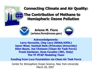
Connecting Climate and Air Quality: The Contribution of Methane to Hemispheric Ozone Pollution. Arlene M. Fiore (arlene.fiore@noaa.gov). Acknowledgments: Larry Horowitz, Chip Levy (NOAA/GFDL) Jason West, Vaishali Naik (Princeton University) Ellen Baum, Joe Chaisson (Clean Air Task Force)

E N D
Connecting Climate and Air Quality: The Contribution of Methane to Hemispheric Ozone Pollution Arlene M. Fiore (arlene.fiore@noaa.gov) Acknowledgments: Larry Horowitz, Chip Levy (NOAA/GFDL) Jason West, Vaishali Naik (Princeton University) Ellen Baum, Joe Chaisson (Clean Air Task Force) Frank Dentener, Kees Cuvelier (JRC, Italy) The TF HTAP Modeling Team Funding from Luce Foundation via Clean Air Task Force Center for Atmosphere Ocean Science, New York University March 28, 2007
The U.S. ozone smog problem is spatially widespread, affecting >100 million people Nonattainment Areas (2001-2003 data) 4th highest daily max 8-hr mean O3> 84 ppbv U.S. EPA, 2006
Radiative forcing of climate (1750 to present):Important contributions from methane and ozone IPCC, 2007
Air quality-Climate Linkage:CH4, O3 are greenhouse gasesCH4 contributes to background O3in surface air Stratospheric O3 Stratosphere O3 ~12 km hn Free Troposphere NO NO2 Hemispheric Pollution OH HO2 Direct Intercontinental Transport Boundary layer (0-3 km) VOC, CH4, CO air pollution (smog) NOx VOC O3 NOx VOC O3 air pollution (smog) CONTINENT 1 CONTINENT 2 OCEAN A.M. Fiore
IPCC [2001] scenarios project future growth Change in 10-model mean surface O3 Projections of future CH4 emissions (Tg CH4) to 2100 2100 SRES A2 - 2000 Attributed mainly to increases in methane and NOx [Prather et al., 2003]
Rising background O3 has implications for attaining air quality standards Pre-industrial background Current background Future background? Recent observational analyses suggest that surface O3 background is rising [e.g. Lin et al., 2000; Jaffe et al., 2003, 2005; Vingarzan, 2004; EMEP/CCC-Report 1/2005 ] Europe seasonal WHO/Europe 8-hr average U.S. 8-hr average 20 40 60 80 100 O3 (ppbv) A.M. Fiore
Ozone abatement strategies evolve as our understanding of the ozone problem advances O3 smog recognized as an URBAN problem:Los Angeles, Haagen-Smit identifies chemical mechanism Smog as REGIONAL problem; role of NOx and biogenic VOCs recognized A GLOBAL perspective: role of intercontinental transport, background Present 1980s 1950s AbatementStrategy: NMVOCs + NOx + CH4?? “Methane (and CO) emission control is an effective way of simultaneously meeting air quality standards and abating global warming” --- EMEP/CCC-Report 1/2005 A.M. Fiore
Double dividend of Methane Controls: Decreased greenhouse warming and improved air quality Number of U.S. summer grid-square days with O3 > 80 ppbv 1995 (base) 50% anth. VOC 50% anth. CH4 50% anth. NOx 2030 A1 2030 B1 Radiative Forcing* (W m-2) 50% anth. CH4 50% anth. NOx 50% anth. VOC 2030 A1 2030 B1 GEOS-Chem Model (4°x5°) CH4 links air quality & climate via background O3 Fiore et al., GRL, 2002
Impacts of O3 precursor reductions on U.S. summer afternoon surface O3 frequency distributions GEOS-Chem Model Simulations (4°x5°) NOx controls strongly decrease the highest O3 (regional pollution episodes) CH4 controls affect the entire O3 distribution similarly (background) Results add linearly when both methane and NOx are reduced Fiore et al., 2002; West & Fiore, ES&T, 2005
Methane trends and linkages with chemistry, climate, and ozone pollution Research Tool: MOZART-2 Global Chemical Transport Model [Horowitz et al., 2003] NCEP, 1.9°x1.9°, 28vertical levels • Fully represent methane-OH relationship Test directly with observations 3D model structure • 1) Climate and air quality benefits from CH4 controls • Characterize the ozone response to CH4 control • Incorporate methane controls into a future emission scenario • 2) Recent methane trends (1990 to 2004) • Are emission inventories consistent with observed CH4 trends? • Role of changing sources vs. sinks? A.M. Fiore
More than half of global methane emissions are influenced by human activities ~300 Tg CH4 yr-1 Anthropogenic [EDGAR 3.2 Fast-Track 2000; Olivier et al., 2005] ~200 Tg CH4 yr-1 Biogenic sources [Wang et al., 2004] >25% uncertainty in total emissions Clathrates? Melting permafrost? PLANTS? 60-240 Keppler et al., 2006 85 Sanderson et al., 2006 10-60 Kirschbaum et al., 2006 0-46 Ferretti et al., 2006 BIOMASS BURNING + BIOFUEL 30 ANIMALS 90 WETLANDS 180 LANDFILLS + WASTEWATER 50 GAS + OIL 60 COAL 30 TERMITES 20 RICE 40 GLOBAL METHANE SOURCES (Tg CH4 yr-1) A.M. Fiore
Surface Methane Abundance (ppb) DTropospheric O3 Burden (Tg) Characterizing the methane-ozone relationship with idealized model simulations Reduce global anthropogenic CH4 emissions by 30% Simulation Year Model approaches a new steady-stateafter 30 years of simulation Is the O3 response sensitive to the location of CH4 emission controls? A.M. Fiore
Enhanced effect in source region <10% other NH source regions < 5% rest of NH <1% most of SH Percentage Difference: DAsia – Duniform DAsia • Target cheapest controls worldwide Change in July surface O3 from 30% decrease in anthropogenic CH4 emissions Globally uniform emission reduction Emission reduction in Asia A.M. Fiore
Decrease in summertime U.S. surface ozone from 30% reductions in anthrop. CH4 emissions MAXIMUM DIFFERENCE (Composite max daily afternoon mean ozone JJA) NO ASIAN ANTH. CH4 Largest decreases in NOx-saturated regions A.M. Fiore
MOZART-2 [West et al., PNAS 2006; this work] TM3 [Dentener et al., ACP, 2005] GISS [Shindell et al., GRL, 2005] GEOS-CHEM [Fiore et al., GRL, 2002] IPCC TAR [Prather et al., 2001] X Tropospheric O3 responds approximately linearly to anthropogenic CH4 emission changes across models Anthropogenic CH4 contributes ~50 Tg (~15%) to tropospheric O3 burden ~5 ppbv to global surface O3 A.M. Fiore
Multi-model study shows similar surface ozone decreases over NH continents when global methane is reduced Full range of 12 individual models EUROPE N. AMER. S. ASIA E. ASIA • >1 ppbv O3 decrease over all NH receptor regions • Consistent with prior studies TF HTAP 2007 Interim report draft available at www.htap.org A.M. Fiore
0.7 1.4 1.9 How much methane can be reduced? (industrialized nations) 10% of anth. emissions 20% of anth. emissions 0 20 40 60 80 100 120 Methane reduction potential (Mton CH4 yr-1) IEA [2003] for 5 industrial sectors Comparison: Clean Air Interstate Rule (proposed NOx control) reduces 0.86 ppb over the eastern US, at $0.88 billion yr-1 West & Fiore, ES&T, 2005
Will methane emissions increase in the future? Anthropogenic CH4 emissions (Tg yr-1) A2 Dentener et al., ACP, 2005 B2 Current Legislation (CLE) Scenario MFR PHOTOCOMP for IPCC AR-4 used CLE, MFR, A2 scenarios for all O3 precursors [Dentener et al., 2006ab; Stevenson et al., 2006; van Noije et al., 2006; Shindell et al., 2006] Our approach: use CLE as a baseline scenario & apply methane controls
Emission Trajectories in Future Scenarios (2005 to 2030) Surface NOx Emissions 2030:2005 ratio 0.3 0.8 1.4 1.9 2.5 Anthropogenic CH4 Emissions (Tg yr-1) CLE Baseline A B C • Control scenarios reduce 2030 CH4 emissions relative to CLE by: • A)-75 Tg (18%) – cost-effective now • -125 Tg (29%) – possible with current technologies • -180 Tg (42%) – requires new technologies • Additional 2030 simulation where CH4 = 700 ppbv (“zero-out anthrop. CH4”) A.M. Fiore
Reducing tropospheric ozone via methane controls decreases radiative forcing (2030-2005) CLE A B C +0.16 Net Forcing +0.08 0.00 -0.08 -0.58 (W m-2) OZONE METHANE CH4=700 ppb Methane Control Scenario More aggressive CH4 control scenarios offset baseline CLE forcing A.M. Fiore
Future air quality improvements from CH4 emission controls Controls on global CH4 reduce incidence of O3 > 70 ppbv USA Cost-effective controls prevent increased occurrence of O3 > 70 ppbv in 2030 relative to 2005 Percentage of model grid-cell days where surface ozone > 70 ppbv Europe 2030 European high-O3 events under CLE emissions scenario show stronger sensitivity to CH4 than in USA A.M. Fiore
Anthrop. CH4 emissions CLE A B Tg yr-1 C Summary: Connecting climate and air quality via O3 & CH4 • CLIMATE AND AIR QUALITY BENEFITS FROM CH4 CONTROL • Independent of reduction location (but depends on NOx) • Target cheapest controls worldwide • Robust response over NH continents across models • ~1 ppbv surface O3 for a 20% decrease in anthrop. CH4 • Complementary to NOx, NMVOC controls • Decreases hemispheric background O3 • Opportunity for international air quality management How well do we understand recent trends in atmospheric methane? How will future changes in emissions interact with a changing climate? A.M. Fiore
Observed trend in surface CH4 (ppb) 1990-2004 Global Mean CH4 (ppb) • Hypotheses for leveling off • discussed in the literature: • 1. Approach to steady-state • 2. Source Changes • Anthropogenic • Wetlands/plants • (Biomass burning) • 3. (Transport) • 4. Sink (CH4+OH) • Humidity • Temperature • OH precursor emissions • overhead O3 columns NOAA GMD Network Data from 42 GMD stations with 8-yr minimum record is area-weighted, after averaging in bands 60-90N, 30-60N, 0-30N, 0-30S, 30-90S Can the model capture the observed trend (and be used for attribution)? A.M. Fiore
Overestimates interhemispheric gradient Mean Bias (ppb) r2 Correlates poorly at high N latitudes S Latitude N Bias and correlation vs. observed surface CH4: 1990-2004 BASE simulation EDGAR 2.0 emissions held constant Global Mean Surface Methane (ppb) OBSERVED MOZART-2 Overestimates 1990-1997 but matches trend Captures flattening post- 1998 but underestimates abundance
Inter-annually varying wetland emissions 1990-1998 from Wang et al. [2004] (Tg CH4 yr-1); different distribution Apply climatological mean (224 Tg yr-1) post-1998 ANTH ANTH + BIO Estimates for changing methane sources in the 1990s Biogenic adjusted to maintain constant total source 547 Tg CH4 yr-1 BASE EDGAR anthropogenic inventory A.M. Fiore
Bias & Correlation vs. GMD CH4 observations: 1990-2004 Global Mean Surface Methane (ppb) Mean Bias (ppb) OBS BASE ANTH ANTH+BIO ANTH+BIOsimulation with time-varying EDGAR 3.2 + wetland emissions improves: Global mean surface conc. Interhemispheric gradient • Correlation at high N latitudes r2 Fiore et al., GRL, 2006 S Latitude N
CH4 Lifetime (t)against Tropospheric OH t = Humidity Photolysis Lightning NOx Temperature (88% of CH4 loss is below 500 hPa ) Dt What drives the change in methane lifetime in the model? Dt = 0.17 yr = 1.6%) How does meteorology influence methane abundances? Why does BASE run with constant emissions level off post-1998? Examine sink A.M. Fiore
+ = Global Lightning NOx (TgN yr-1) DT(+0.3K) BASE DOH(+1.2%) An increase in lightning NOx drives the OH increase in the model But lightning NOx is highly parameterized …how robust is this result? Small increases in temperature and OH shorten the methane lifetime against tropospheric OH DtOH Deconstruct Dt (-0.17 years) from 1991-1995 to 2000-2004 into individual contributions by varying OH and temperature separately A.M. Fiore
Donner RAS MOZART LIS/OTD Flash counts Magnetic field variations in the lower ELF range [e.g. Williams, 1992; Füllekrug and Fraser- Smith, 1997; Price, 2000] free-running GCM Lightning NOx increase robust; magnitude depends on meteorology Negev Desert Station, Israel Additional evidence for a global lightning NOx increase? • Estimate lightning NOx changes using options available in the GFDL Atmospheric General Circulation Model: • Convection schemes (RAS vs. Donner-deep) • Meteorology (free-running vs. nudged to NCEP reanalysis) • More physically-based lightning NOx scheme [Petersen et al., 2005] • Evidence from observations? Lightning NOx % change (91-95 to 00-04) NCEP(nudged) c/o L.W. Horowitz A.M. Fiore
Methane (ppb) • METHANE TRENDS FROM 1990 TO 2004 • Simulation with time-varying emissions and meteorology • best captures observed CH4 distribution • Model trend driven by increasing T, OH • Trends in global lightning activity? • Potential for climate feedbacks (on sources and sinks) OBS BASE ANTH ANTH+BIO Anthrop. CH4 emissions CLE A DtOH91-95 to 01-04 B Tg yr-1 C + = DT DOH BASE Summary: Connecting climate and air quality via O3 & CH4 • CLIMATE AND AIR QUALITY BENEFITS FROM CH4 CONTROL • Independent of reduction location (but depends on NOx) • Target cheapest controls worldwide • Robust response over NH continents across models • ~1 ppbv surface O3 for a 20% decrease in anthrop. CH4 • Complementary to NOx, NMVOC controls • Decreases hemispheric background O3 • Opportunity for international air quality management A.M. Fiore