Inferences On Two Samples
Inferences On Two Samples. Overview. We continue with confidence intervals and hypothesis testing for more advanced models Models comparing two means When the two means are dependent When the two means are independent Models comparing two proportions. Inference about Two Means:

Inferences On Two Samples
E N D
Presentation Transcript
Overview • We continue with confidence intervals and hypothesis testing for more advanced models • Models comparing two means • When the two means are dependent • When the two means are independent • Models comparing two proportions
Inference about Two Means: Dependent/paired Samples
Learning Objectives • Distinguish between independent and dependent sampling • Test hypotheses made regarding matched-pairs data • Construct and interpret confidence intervals about the population mean difference of matched-pairs data
Two populations • So far, we have covered a variety of models dealing with one population • The mean parameter for one population • The proportion parameter for one population • However, there are many real-world applications that need techniques to compare two populations
Examples • Examples of situations with two populations • We want to test whether a certain treatment helps or not … the measurements are the “before” measurement and the “after” measurement • We want to test the effectiveness of Drug A versus Drug B … we give 40 patients Drug A and 40 patients Drug B … the measurements are the Drug A and Drug B responses
Dependent Sample • In certain cases, the two samples are very closely tied to each other • A dependentsample is one when each individual in the first sample is directly matched to one individual in the second • Examples • Before and after measurements (a specific person’s before and the same person’s after) • Experiments on identical twins (twins matched with each other
Independent Sample • On the other extreme, the two samples can be completely independent of each other • An independentsample is when individuals selected for one sample have no relationship to the individuals selected for the other • Examples • Fifty samples from one factory compared to fifty samples from another • Two hundred patients divided at random into two groups of one hundred
Paired Samples • The dependent samples are often called matched-pairs • Matched-pairs is an appropriate term because each observation in sample 1 is matched to exactly one in sample 2 • The person before the person after • One twin the other twin • An experiment done on a person’s left eye the same experiment done on that person’s right eye
Analysis of Paired Samples • The method to analyze matched-pairs is to combine the pair into one measurement • “Before” and “After” measurements – subtract the before from the after to get a single “change” measurement • “Twin 1” and “Twin 2” measurements – subtract the 1 from the 2 to get a single “difference between twins” measurement • “Left eye” and “Right eye” measurements – subtract the left from the right to get a single “difference between eyes” measurement
Compute Difference d • Specifically, for the before and after example, • d1 = person 1’s after – person 1’s before • d2 = person 2’s after – person 1’s before • d3 = person 3’s after – person 1’s before • This creates a new random variable d • We would like to reformulate our problem into a problem involving d (just one variable)
Test for the True Difference μd • How do our hypotheses translate? • The two means are equal -> the mean difference is zero -> μd = 0 • The two means are unequal -> the mean difference is non-zero -> μd ≠ 0 • Thus our hypothesis test is • H0: μd = 0 • H1: μd ≠ 0 • The standard deviation σd is unknown • We know how to do this!
Test for the True Difference • To solve • H0: μd = 0 • H1: μd ≠ 0 • The standard deviation σd is unknown • This is exactly the test of one population mean with the standard deviation being unknown • This is exactly the subject covered in Unit 8
Assumptions • In order for this test statistic to be used, the data must meet certain conditions • The sample is obtained using simple random sampling • The sample data are matched pairs • The differences are normally distributed, or the sample size (the number of pairs, n) is at least 30 • These are the usual conditions we need to make our Student’s t calculations
Example • An example … whether our treatment helps or not … helps meaning a higher measurement • The “Before” and “After” results
Example (continued) • Hypotheses • H0: μd = 0 … no difference • H1: μd > 0 … helps • (We’re only interested in if our treatment makes things better or not) • α = 0.01 • Calculations • n = 5 (i.e. 5 pairs) • = .88 (mean of the paired-difference) • sd = .83
Example (continued) • Calculations • n = 5 • d = 0.88 • sd = 0.83 • The test statistic is • This has a Student’s t-distribution with 4 degrees of freedom
Example (continued) • Use the Student’s t-distribution with 4 degrees of freedom • The right-tailed α = 0.01 critical value is 3.75 (i.e. t0.01;4 d.f. = 3.75) • 2.36 is less than 3.75 (the classical method) • Thus we do not reject the null hypothesis • There is insufficient evidence to conclude that our method significantly improves the situation • We could also have used the P-Value method. P value is 0.039 (note: tcdf(2.36, E99, 4) = 0.039)
Example (continued) • Matched-pairs tests have the same various versions of hypothesis tests • Two-tailed tests • Left-tailed tests (the alternatively hypothesis that the first mean is less than the second) • Right-tailed tests (the alternatively hypothesis that the first mean is greater than the second) • Each can be solved using the Student’s t
Classical and P-value Approaches • Each of the types of tests can be solved using either the classical or the P-value approach
Summary of the Method • A summary of the method • For each matched pair, subtract the first observation from the second • This results in one data item per subject with the data items independent of each other • Test that the mean of these differences is equal to 0 • Conclusions • Do not reject that μd = 0 • Reject that μd = 0 ... Reject that the two populations have the same mean
Construct and interpret confidence intervals about the population mean difference of matched-pairs data
Confidence Interval for the Paired Difference • We’ve turned the matched-pairs problem in one for a single variable’s mean / unknown standard deviation • We just did hypothesis tests • We can use the techniques taught in Unit 7 (again, single variable’s mean / unknown standard deviation) to construct confidence intervals • The idea – the processes (but maybe not the specific calculations) are very similar for all the different models
Confidence Interval for the Paired Difference • Confidence intervals are of the form Point estimate ± margin of error • This is precisely an application of our results for a population mean / unknown standard deviation • The point estimate d and the margin of error for a two-tailed test
Confidence Interval for the Paired Difference • Thus a (1 – α) • 100% confidence interval for the difference of two means, in the matched-pair case, is where tα/2 is the critical value of the Student’st-distribution with n – 1 degrees of freedom
Example Salt-free diets are often prescribed for people with high blood pressure. The following data was obtained from an experiment designed to estimate the reduction in diastolic blood pressure as a result of following a salt-free diet for two weeks. Assume diastolic readings to be normally distributed. Find a 99% confidence interval for the mean reduction
3. Sample evidence Sample information: Example (continued) 1. Population Parameter of InterestThe mean reduction (difference) in diastolic blood pressure 2. The Confidence Interval Criteria a. Assumptions: Both sample populations are assumed normal b. Test statistic: t with df = 8 - 1 = 7 c. Confidence level: 1 -a = 0.99
Example 4. The Confidence Interval a. Confidence coefficients: Two-tailed situation, a/2 = 0.005t(df, a/2) = t(7, 0.005) = 3.50 b. Maximum error: c. Confidence limits: 5. The Results -1.957 to 3.957 is the 99% confidence interval estimate for the amount of reduction of diastolic blood pressure, md..
Summary • Two sets of data are dependent, or matched-pairs, when each observation in one is matched directly with one observation in the other • In this case, the differences of observation values should be used • The hypothesis test and confidence interval for the difference is a “mean with unknown standard deviation” problem, one which we already know how to solve
Inference about Two Means: Independent Samples
Learning Objectives • Test hypotheses regarding the difference of two independent means • Construct and interpret confidence intervals regarding the difference of two independent means
Independent Samples • Two samples are independent if the values in one have no relation to the values in the other • Examples of not independent • Data from male students versus data from business majors (an overlap in populations) • The mean amount of rain, per day, reported in two weather stations in neighboring towns (likely to rain in both places)
Independent Samples • A typical example of an independent samples test is to test whether a new drug, Drug N, lowers cholesterol levels more than the current drug, Drug C • A group of 100 patients could be chosen • The group could be divided into two groups of 50 using a random method • If we use a random method (such as a simple random sample of 50 out of the 100 patients), then the two groups would be independent
Test of Two Independent Samples • The test of two independent samples is very similar, in process, to the test of a single population mean • The only major difference is that a different test statistic is used • We will discuss the new test statistic through an analogy with the hypothesis test of one mean
Test hypotheses regarding the difference of two independent means
Test Statistic for a Single Mean • For the test of one mean, we have the variables • The hypothesized mean (μ) • The sample size (n) • The sample mean (x) • The sample standard deviation (s) • We expect that x would be close to μ
Test statistic for the Difference of Two Means • In the test of two means, we have two values for each variable – one for each of the two samples • The two hypothesized means μ1and μ2 • The two sample sizes n1 and n2 • The two sample means x1 and x2 • The two sample standard deviations s1 and s2 • We expect that x1 – x2 would be close to μ1 – μ2
Standard Error of the Test Statistic for a Single Mean • For the test of one mean, to measure the deviation from the null hypothesis, it is logical to take x – μ which has a standard deviation/standard error of approximately
Standard Error of the Test Statistic for the Difference of Two Means • For the test of two means, to measure the deviation from the null hypothesis, it is logical to take (x1 – x2) – (μ1 – μ2) which has a standard deviation/standard error of approximately
t -Test Statistic for a Single Mean • For the test of one mean, under certain appropriate conditions, the difference x – μ is Student’s t with mean 0, and the test statistic has Student’s t-distribution with n – 1 degrees of freedom
t - Test Statistic for the Difference of Two Means • Thus for the test of two means, under certain appropriate conditions, the difference (x1 – x2) – (μ1 – μ2) is approximately Student’s t with mean 0, and the test statistic has an approximate Student’s t-distribution
Distribution of the t-statistic • This is Welch’s approximation, that has approximately a Student’s t-distribution • The degrees of freedom is the smaller of n1 – 1 and n2 – 1 Note: Some computer or calculator calculates the degrees of freedom for this t test statistic with a somewhat complicated formula. But, we’ll use the smaller of n1 – 1 and n2 – 1 as the degrees of freedom.
A Special Case • For the particular case where be believe that the two population means are equal, or μ1 = μ2, and the two sample sizes are equal, or n1 = n2, then the test statistic becomes with n – 1 degrees of freedom, where n = n1 = n2
General Test Procedure • Now for the overall structure of the test • Set up the hypotheses • Select the level of significance α • Compute the test statistic • Compare the test statistic with the appropriate critical values • Reach a do not reject or reject the null hypothesis conclusion
Assumptions • In order for this method to be used, the data must meet certain conditions • Both samples are obtained using simple random sampling • The samples are independent • The populations are normally distributed, or the sample sizes are large (both n1 and n2 are at least 30) • These are the usual conditions we need to make our Student’s t calculations
State Hypotheses & level of significance • State our two-tailed, left-tailed, or right-tailed hypotheses • State our level of significance α, often 0.10, 0.05, or 0.01
Compute the Test Statistic • Compute the test statistic and the degrees of freedom, the smaller ofn1 – 1 and n2 – 1 • Compute the critical values (for the two-tailed, left-tailed, or right-tailed test
Make a Statistical Decision • Each of the types of tests can be solved using either the classical or the P-value approach • Based on either of these methods, do not reject or reject the null hypothesis
Example • We have two independent samples • The first sample of n = 40 items has a sample mean of 7.8 and a sample standard deviation of 3.3 • The second sample of n = 50 items has a sample mean of 11.6 and a sample standard deviation of 2.6 • We believe that the mean of the second population is exactly 4.0 larger than the mean of the first population • We use a level of significance α = .05 • We test versus


