Download
1 / 22
220 likes | 368 Vues
Energy Optimal Control for Time Varying Wireless Networks. Michael J. Neely University of Southern California http://www-rcf.usc.edu/~mjneely. S={Totally Awesome}. Power Vector: P(t) = (P 1 (t), P 2 (t), …, P L (t)).

E N D
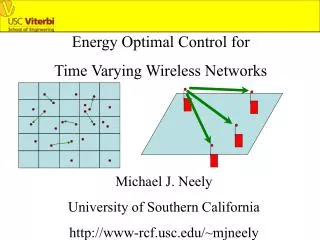
Energy Optimal Control for Time Varying Wireless Networks Michael J. Neely University of Southern California http://www-rcf.usc.edu/~mjneely
S={Totally Awesome} Power Vector: P(t) = (P1(t), P2(t), …, PL(t)) Channel States: S(t) = (S1(t), S2(t), …, SL(t)) (i.i.d. over slots) m(P(t), S(t)) Rate-Power Function: (where P(t)P for all t) Part 1: A single wireless downlink (L links) L 2 1 Slotted time t = 0, 1, 2, … t 0 1 2 3 …
A1(t) A2(t) AL(t) S={Totally Awesome} Random arrivals : Ai(t) = arrivals to queue i on slot t (bits) Queue backlog : Ui(t) = backlog in queue i at slot t (bits) mL(P(t), S(t)) m2(P(t), S(t)) m1(P(t), S(t)) Rate vector: l = (l1, l2, …, lL) (potentially unknown) Arrivals and channel states i.i.d. over slots (unknown statistics) Arrival rate: E[Ai(t)] = li (bits/slot), i.i.d. over slots Allocate power in reaction to queue backlog + current channel state…
A1(t) A2(t) AL(t) S={Totally Awesome} Random arrivals : Ai(t) = arrivals to queue i on slot t (bits) Queue backlog : Ui(t) = backlog in queue i at slot t (bits) P(t)P) mL(P(t), S(t)) m2(P(t), S(t)) m1(P(t), S(t)) (both have peak power constraint: Two formulations: 1. Maximize thruput w/ avg. power constraint: 2. Stabilize with minimum average power (will do this for multihop)
Some precedents: Energy optimal scheduling with known statistics: -Li, Goldsmith, IT 2001 [no queueing] -Fu, Modiano, Infocom 2003 [single queue] -Yeh, Cohen, ISIT 2003 [downlink] -Liu, Chong, Shroff, Comp. Nets. 2003 [no queueing, known stats or unknown stats approx] Stable queueing w/ Lyapunov Drift: MWM -- max miUi policy -Tassiulas, Ephremides, Aut. Contr. 1992 [multi-hop network] -Tassiulas, Ephremedes, IT 1993 [random connectivity] -Andrews et. Al. , Comm. Mag. 2001 [server selection] -Neely, Modiano, TON 2003, JSAC 2005 [power alloc. + routing] (these consider stability but not avg. energy optimality…)
A1(t) A2(t) m1(t) m2(t) Example: Can either be idle, or allocate 1 Watt to a single queue. S1(t), S2(t) {Good, Medium, Bad}
P(t)P L = Region of all supportable input rate vectors l Capacity region L of the wireless downlink: (i) Peak power constraint: l1 l2 • Capacity region L assumes: • Infinite buffer storage • -Full knowledge of future arrivals and channel states
P(t)P L = Region of all supportable input rate vectors l Capacity region L of the wireless downlink: (i) Peak power constraint: l1 (ii) Avg. power constraint: l2 • Capacity region L assumes: • Infinite buffer storage • -Full knowledge of future arrivals and channel states
P(t)P L = Region of all supportable input rate vectors l Capacity region L of the wireless downlink: (i) Peak power constraint: l1 (ii) Avg. power constraint: l2 • Capacity region L assumes: • Infinite buffer storage • -Full knowledge of future arrivals and channel states
A1(t) A2(t) AL(t) X(t+1) = max[X(t) - Pav, 0] + Pi(t) P(t)P mL(P(t), S(t)) m2(P(t), S(t)) L L m1(P(t), S(t)) i=1 i=1 Pav Observation: If we stabilize all original queues and the virtual power queue subject to only the peak power constraint , then the average power constraint will automatically be satisfied. Pi(t) To remove the average power constraint , we create a virtual power queue with backlog X(t). Dynamics:
X(t+1) = max[X(t) - Pav, 0] + Pi(t) L i=1 Control policy: In this slide we show special case when P restricts power options to full power to one queue, or idle (general case in paper). A1(t) A2(t) AL(t) m1(t) m2(t) mL(t) Ui(t)mi(t) - X(t)Ptot Choose queue i that maximizes: Whenever this maximum is positive. Else, allocate no power at all. Then iterate the X(t) virtual power queue equation:
Theorem: Finite buffer size B, input rate l L or l L L L ri* ri - C/(B - Amax) i=1 i=1 Performance of Energy Constrained Control Alg. (ECCA): (r1*,…, rL*) = optimal vector (r1, …, rL) = achieved thruput vec. (a) Thruput: (b) Total power expended over any interval(t1, t2) Pav(t2-t1) + Xmax where C, Xmax are constants independent of rate vector and channel statistics. C = (Amax2 + Ppeak2 + Pav2)/2
(Assume (lic) L) N j n=1 Goal: Develop joint routing, scheduling, power allocation to minimize E[gi( Pij)] (where gi( ) are arbitrary convex functions) Part 2: Minimizing Energy in Multi-hop Networks N node ad-hoc network (lic) = input rate matrix = (rate from source i to destination node j) Sij(t) = Current channel state between nodes i,j
(Assume (lic) L) N j n=1 Goal: Develop joint routing, scheduling, power allocation to minimize E[gi( Pij)] To facilitate distributed implementation, use a cell-partitioned model… Part 2: Minimizing Energy in Multi-hop Networks N node ad-hoc network (lic) = input rate matrix = (rate from source i to destination node j) Sij(t) = Current channel state between nodes i,j
(Assume (lic) L) N j n=1 Goal: Develop joint routing, scheduling, power allocation to minimize E[gi( Pij)] To facilitate distributed implementation, use a cell-partitioned model… Part 2: Minimizing Energy in Multi-hop Networks N node ad-hoc network (lic) = input rate matrix = (rate from source i to destination node j) Sij(t) = Current channel state between nodes i,j
L(U(t)) = Un2(t) + Vg(P (t)) - Vg(P *) n n n D(t) = E[L(U(t+1) - L(U(t)) | U(t)] E[Un] + C/V E[g(P )] C + VGmax g(P*) e Analytical technique: Lyapunov Drift Lyapunov function: Lyapunov drift: Theorem: (Lyapunov drift with Cost Minimization) If for all t: D(t) C - e Un(t) Then: (a) (stability and bounded delay) (b) (resulting cost)
cl*(t) = ( Joint routing, scheduling, power allocation: link l (similar to the original Tassiulas differential backlog routing policy [92])
li* lj* (2) Each node computes its optimal power level Pi* for link l from (1): Pi* maximizes: ml(P, Sl(t))Wl* - Vgi(P) (over 0 < P < Ppeak) Qi* (3) Each node broadcasts Qi* to all other nodes in cell. Node with largest Qi* transmits: Transmit commodity cl* over link l*, power level Pi*
Performance: e e e = “distance” to capacity region boundary. Theorem: If e>0, we have…
A1(t) A2(t) m1(t) m2(t) Example Simulation: Two-queue downlink with {G, M, B} channels
Conclusions: Virtual power queue to ensure average power constraints. Channel independent algorithms (adapts to any channel). Minimize average power over multihop networks over all joint power allocation, routing, scheduling strategies. 4. Stochastic network optimization theory
http://www-rcf.usc.edu/~mjneely/ the end