Ch. 2 Algorithms for Systems of Linear Equations

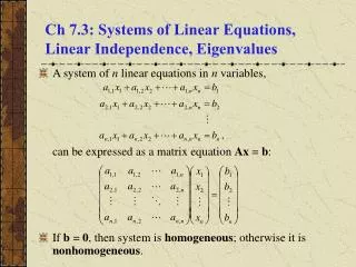
EE692 Parallel and Distribution Computation | Prof. Song Chong Ch. 2 Algorithms for Systems of Linear Equations

Overview • Consider the system of linear equations A: n x n real matrix, b: vector in Rn • Direct method to find “exact” solution (sec 2.1~2.3) with a finite number of operations, typically of the order of n3 e.g.) Gaussian Elimination

Overview (Cont’d) • Iterative methods do not obtain an exact solution of Ax = b in finite time, but they converge to a solution asymptotically • Often yield a solution, within acceptable precision, after a relatively small number of iterations • Usually preferred when n is very large • May have smaller storage requirement than direct methods • Performance measures • Direct method: complexity • Iteration method: speed of convergence e.g.) geometrical convergence

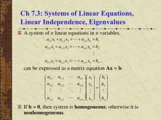
Classical Iterative Methods • Assume that A is invertible so that Ax = b has a unique solution. Write the i-th equation as • Assuming aii≠0 and solving for xi, ------(1) • If xj, j≠i, (or estimates) are known (available), one can obtain xi (or an estimate of xi)

Jacobi Algorithm • Starting with some initial vector , evaluate x(t), t=1,2,..., using the iteration • If the sequence {x(t)} converges to a limit x*, then obviously x* satisfies Eg.(1) for each i. • Condition for Convergence?? e.g.) >> Case 1: Convergence case >> Case 2: Divergence case

Jacobi Algorithm (Cont’d) • Convergence Case Divergence Case

Gauss-Seidel Algorithm • Starting with • Any other order of updating is possible • Different order of updating may produce substantially different results for the same problem

Relaxation of Iterative Methods • Relaxation of Eq.(1) using relaxation parameter • Jacobi overrelaxation (JOR) • Convex computation of xi(t) and Jacobi iteration • Gauss-Seidel overrelaxation (SOR) • Convex combination of xi(t) and Gauss-Seidel iteration • JOR and SOR are widely used because they often converge faster if is suitably chosen

Richardson’s method • Following equation is obtained by rewriting • Richardson-Gauss-Seidel [RGS] method • A more general form using an invertible matrix B

Parallel Implementation • Jacobi, JOR and Richardson’s algorithms are straightforward to implement in parallel • Gauss-Seidel, SOR and RGS algorithms are not well suited for parallel implementation in general because they are inherently sequential • Typical termination criteria used in practice

Applications: Poisson’s equation • Find a function f:[0,1]2R that satisfies where g:[0,1]2R is a known function and f has prescribed values on the boundary of the unit square. • Let

Applications: Poisson’s equation (cont’d) • Assume that f is sufficiently smooth and the is a small scalar, by Prop. A.33 in Appendix A. • By plugging (2) and (3) into (1), • A system of (N-1)2 linear equations in (N-1)2 unknowns, i.e., can be represented in the form Ax=b.

Applications: Poisson’s equation (cont’d) • JOR algorithm where fi,j(t)=fi,j are known, whenever i or j is equal to 0 or N.

Applications: Power Control of CDMA Uplink • Assume K users in a cell, SINR per chip, denoted by SINRc, of user i is where is the received energy per chip for user i and N0 is noise. • Since each bit is encoded onto a pseudonoise sequence of length Gi chips at the transmitter, the received energy per bit for user i is .

Applications: Power Control of CDMA Uplink (cont’d) • The SINR of user i, or equivalently the ratio of the received energy per bit to the interference and noise per chip (commonly called in the CDMA literature) is where pi (joules/sec) is the transmit power of user i and gi is the attenuation of user i’s signal to base station.

Applications: Power Control of CDMA Uplink (cont’d) • To achieve equally reliable communication, where is a certain threshold. • The data rate of user i, Ri (bits/sec), is and Gi is called the processing gain of user i.

Applications: Power Control of CDMA Uplink (cont’d) • The power control problem of CMDA uplink is to find minimal nonnegative transmit power vector satisfying That is, find nonnegative satisfying • A system of K linear equations in K unknowns, i.e., can be represented in the form Ax=b.

Applications: Power Control of CDMA Uplink (cont’d) • JOR algorithm For each user i, where β, Gi, gi, N0 and W are given.

Parallelization of Iterative Methods Using Dependency Graph • Consider a Jacobi-type iteration in the general form • The communication required for this iteration can be described by means of a directed graph G=(N,A), called the dependency graph. • The set of nodes N is {1,…,n}, corresponding to the components of x. Let (i,j) be an arc of the dependency graph if and only if the function fj depends on xi.

Parallelization of Iterative Methods Using Dependency Graph (cont’d) • The dependency over iterations can be described by means of a directed acyclic graph (DAG) where the nodes one of the form (i,t) and arcs are of the form ((i,t), (j,t+1)). t=0 The depth of the single iteration (sweep) is 1 t t=1 t=2

Parallelization of Iterative Methods Using Dependency Graph (cont’d) • Consider a Gauss-Seidel type iteration in the general form • Often preferable since it incorporates the newest available information, thereby sometimes converging faster than the Jacobi type • Maybe completely non-parallelizable since it is sequential in nature • When the dependency graph is sparse, it is possible that certain component updates can be parallelized • The degree of parallelism may depend on update ordering e.g.) ordering 1234 The depth of the single iteration (sweep) is 3

Parallelization of Iterative Methods Using Dependency Graph (cont’d) The depth of the single iteration is 2 • Finding an optimal update ordering that maximizes parallelisms in Gauss-Seidel algorithm is equivalent to an optimal coloring problem. e.g.) ordering 1342

Parallelization of Iterative Methods Using Dependency Graph (cont’d) • Given the dependency graph G=(N,A), a coloring of G, using K colors, is defined as a mapping h:N->{1,…, K} that assigns a color k=h(i) to each node i in N. • Prop. 2.5 There exists an ordering such that a sweep of the Gauss-Seidel algorithm can be performed in K parallel steps if and only if there exists a coloring of the dependency graph that uses K colors and with the property that there exists no positive cycle with all nodes on the cycle having the same color. • Prop. 2.6 Suppose that if and only if . Then, there exists an ordering such that a sweep of the Gauss-Seidel algorithm can be performed in K parallel steps if and only if there exists a coloring of the dependency graph that uses at most K colors and such that adjacent nodes have different colors. • Unfortunately, the optimal coloring problems are intractable, i.e., there is know known efficient algorithm for solving them.

Convergence Analysis of Classical Iterative Methods • Prop. 4.1 If , generated by any of the above presented algorithms converges, then it converges to a solution of .

Uniform representation of the different algorithms • Let B = A-D where D is a diagonal matrix whose entries are equal to the corresponding diagonal entries of A. • Assuming that the diagonal entries of A are nonzero, the Jacobi algorithm can be written as • Similarly, the JOR <Jacobi> <JOR>

Uniform representation of the different algorithms (cont’d) Decompose A=L+D+U where L strictly lower triangular D diagonal U strictly upper triangular Then, the Gauss-Seidel can be written as <Gauss-Seidel>

iterative matrix Uniform representation of the different algorithms (cont’d) Similarly, Finally, The uniform representation is <SOR> <Richardson>

Uniform representation of the different algorithms (cont’d) • Assume that I-M is invertible (fact: A invertible and nonzero diagonal  I-M invertible for all the algorithm Ex.6.1). Then, there exists a unique x* satisfying x* = Mx* + Gb. • Let y(t) = x(t) – x*. Then, • The solution form is then for every t. • Y(t)  0 iff Mt  0 iff all the eigenvalue of M have a magnitude smaller than 1, i.e., the spectral radius .

Uniform representation of the different algorithms (cont’d) • Prop. 6.1 Assume that I-M is invertible, let x* satisfy x*=Mx*+Gb and let {x(t)} be the sequence generated by the iteration x(t+1) = Mx(t) + Gb. Then, • Note : G and b are nothing to do with convergence • Proof) to be done!

Ch. 2 Algorithms for Systems of Linear Equations