R-TREES
R-TREES. CMPE 422:Database systems Ahmet Menteş. TOPICS COVERED. Introduction Spatial Data and Queries R-Tree Index Algorithms and Complexities Performance R-Tree Variations Conclusion. INTRODUCTION. First Proposed By Antonin Guttman, 1984 from UC Berkeley

R-TREES
E N D
Presentation Transcript
R-TREES CMPE 422:Database systems Ahmet Menteş
TOPICS COVERED • Introduction • Spatial Data and Queries • R-Tree Index • Algorithmsand Complexities • Performance • R-Tree Variations • Conclusion
INTRODUCTION • First Proposed By Antonin Guttman, 1984 from UC Berkeley -“A Dynamic Index Structure For Spatial Searching” • R-Tree structures are used for effectively storing and indexing spatial data. Usage areas are wide • -Computer Aided Design-CAD • -Video Recognition-VR • -Image Processing
INTRODUCTION • R-Trees have correspondance with B-Trees but used for keeping spatial data. -Based on B-trees • B-Trees cannot store new types of data • Wanted to store geometrical data and multi-dimensional data • Region-trees (R-trees)
SPATIAL DATA • Any Type of Geometry • Point • City • Line • Trail • Polygon • Border • A Collection of Geometries • Ski Resort Trails • Any Coordinate System • Meters • Pixels • WGS84 (GPS)
SPATIAL QUERY TYPES • Standard Insert, Search and Delete Queries • Spatial Range Queries • Find all cities within 30 kmof İstanbul • Nearest Neighbor Queries • Find the closest restourants to my address • Spatial Join Queries • Find all neighborhoods that are within 5 km of a university • Geometry Set Operations • Equal(), Disjoint(), Intersect(), Touch(), Cross(), Within(), Contains(), Overlap(), Distance(), Intersection(), Union(), Difference() and more...
R-TREE • R-tree is a depth-balanced tree –Each node corresponds to a disk page –Leaf node: an array of leaf entries A leaf entry: (mbb,oid) –Non-leaf node: an array of node entries A node entry: (dr, nodeid)
R-TREE INDEX STRUCTURE • Data objects in the map are represented by the Minimum Bounding Rectangles (MBRs)
R-TREE INDEX STRUCTURE Formal Description • Structure consisting of (regular) nodes containing tuples <I, child-pointer> • At the lowest level: leaf-nodes with tuples <I, tuple-identifier> • I = (I0, I1, … In) corresponds to MBR • n = Number of Dimensions in the Geometry • Each I is a set of the form [a,b] describing the range of the rectangle along the dimension • a or b can be equal to infinity • Tuple-identifier points to a record
R-TREE INDEX STRUCTURE • Important Parameters for R-Tree index • M is the maximum number of entries in one node • Parameter m ≤ M/2 specifies the minimum number of entries in a node • Every Leaf Node Contains Between m and M index records unless it is root. • For each index record, <I, tuple-identifier> in a leaf node is the smallest rectangle that spatially contains the n-dimensional data object. • Every non-leaf node has between m and M children unless it is the root. • For each entry <I, child-pointer> in a non-leaf node, I is the smallest rectangle that spatially contains the rectangles in the child nodes. • The root node has at least two children unless it is a leaf. • All leaves appear on the same level. • Height of an R-Tree logmN-1
ALGORITHMS OVERVIEW • For all queries, it is possible to check if a point is within a rectangle in linear time (O(n)). • Query Types To Be Reviewed • Search • Splitting • Insertion • Deletion • Nearest Neighbor
SEARCH • Similar to B-tree search • Quite easy & straight forward(Traverse the whole tree starting at theroot node) • No guarantee on good worst-case performance!(Possible overlapping of rectangles of entries within a single node!)
SEARCH • For all entries in a non-leaf node: Check if overlapping If yes: check node pointed to by this entry. • If node is a leaf-node: Check all entries if overlapping the search object If yes: entry is a qualifying record!
SEARCH COMPLEXITY • Worst Case • Linear Search • Every MBR overlaps the search area • Best Case • No more than one overlap at each level • Complexity becomes O(logMn) • Again, dependent on geometries
SPLITTING • Splitting of nodes necessary afterunderflow oroverflow (as a result of a delete or insert operation) • Ultimate goal: Minimize the resulting node’s MBRs • Secondary aim: Speed of algorithm • 3 Implementations to split an R-Tree: Exhaustive, Quadratic-cost, Linear-cost
SPLITTING • Minimal resulting MBRs: • Exhaustive Approach: • Simply try all possible split-ups but this kind of approach is very costly in terms of complexity issue.
SPLITTING • Quadratic-cost Algorithm: • Pick the 2 out of M entries that would consume the most space if put together. Put one in each group • For all remaining entries: Pick the one that would makethe biggest difference in area when put to one of the two groups. Add it to the one with the least difference • Finished when all entries are put in either group! • Quadratic in M, linear in the number of dimensions.
SPLITTING • Linear-cost Implementation: • Basically the same as quadratic-cost algorithm • Differences: First pair is picked by finding the two rectangles with the greatest normalizedseparation in anydimension. Remaining pairs are selected randomly. • Linear in M as well as in the number ofdimensions
INSERTION • Similar to corresponding B-tree operation • Basically consist of 3 parts: 1. CHOOSELEAF (Find place to insert new object) 2. INSERT (Insert the new object) 3. ADJUSTTREE (Adjusting preceding nodes)
INSERTION Description: • CHOOSELEAF: • Start with root and run through all nodes then; • Find the one which would have to be leastenlarged to include given object! • INSERT: • Check if room for another entry Insert new entry directly OR after callingSPLITNODE (in case of no room)
INSERTION • ADJUSTTREE: • Ascend from node with new entry: • Adjust all MBRs! • In case of node split: • Add new entry to parent node(If no room in parent node, invokeSPLITNODE again) • Propagate upwards till root is reached!
INSERTION COMPLEXITY • IMPORTANT: Make sure nodes are split so they cover the smallest possible area. • Minimize search time • Important variables • N = Number of entries in each node • T = Tree height • Worst Case • 2 * N * T • O(n) GOOD SPLIT! BAD!
DELETION • NOT similar to B-tree DELETE (Treatment of underflows) • B-tree: Merge under-full node with “neighbor” • R-tree: Delete under-full node and re-insert • Why? Re-use of INSERT routine Incrementally refines spatial structure
DELETION Description • FINDLEAF: • Locate the leaf that contains object to be deleted • DELETE: • Delete entry from node • CONDENSETREE: • If node with the removed entry has too few entries, reallocate them • Recursively check the parent nodes until reaching the root • Update all MBR and remove all nodes that underfull • Reinsert all entries removed from the removed nodes according to the INSERT algorithm.
DELETION COMPLEXITY • Deletion variables • N = number of entries in each node • T = tree height • Complexity • 2 * N * T
NEAREST NEIGHBOR • Two Options • Branch-and-bound search • Best first search • Branch-and-bound • Find two distances to each object • Minimum distance from the search point to any side of the other object’s MBR • Minmax distance • Least of the furthest distance in every dimension • Lowest upper bound on the distance from the point to an object • Best First Search • Calculates minmax distance for all objects • R-Tree sorted by minmax distance • Removes nodes from sorted tree • If node has no children it is the nearest neighbor.
NEAREST NEIGHBOR • Branch-and-Bound • Takes longer because it searches all nodes that have not been pruned • Best First Search • Investigates only the closest nodes • Large priority queue data structure in memory • Can cause thrashing • Run-time complexity subject to geometries • How many overlap and how large
PERFORMANCE Why do Benchmarking? • Proof practicality of the structure • Find suitable values for m and M • Test various node-splitting algorithms Testing environment: • C-implementation running under UNIX • Layout of a RISC-II chip with 1057 rectangles • Different page sizes (128 – 2048 bytes) • Various values for M (6 – 102)
PERFORMANCE • Linear INSERT fastest • Linear INSERT quite insensitive to M and m • Quadratic INSERT depends on M as well as m • DELETE extremely sensitive to m
PERFORMANCE • Same page hit / miss performance for linear and quadratic split • Slight advantage for exhaustive version • Space usage strongly depending on m
PERFORMANCE • Quadratic-cost splitting with jumps at INSERT operations for increasing amount of data • Linear INSERT extremely constant • R-tree structure very effective in directing search to small subtrees
R-TREE VARIATIONS R+-Tree: • R+ trees differ from R trees in that: • Nodes are not guaranteed to be at least half filled • The entries of any internal node do not overlap • An object ID may be stored in more than one leaf node. • Advantages • Because nodes are not overlapped with each other, point query performance benefits since all spatial regions are covered by at most one node. • A single path is followed and fewer nodesare visited than with the R-tree. • Disadvantages • Since rectangles are duplicated, an R+ tree can be larger than an R tree built on same data set. • Construction and maintenance of R+ trees is more complex than the construction and maintenance of R trees and other variants of the R tree. R-Tree MBRs R+-Tree MBRs
R-TREE VARIATIONS • R*-Tree • Do not split nodes on insert • Take entries from the overfull node and reinsert them into the tree • Changes MBRs • Saves time and possibly rebalances the tree
CONCLUSION Reasons for R-trees: • Importance of being able to store and effectively search spatial data. • Strong limitations with most spatialstructures (e.g.point data only, not dynamic, performance with paged memory, …) Basic Idea: • Structure similar to B-tree. • Represent objects by their MBR. • Allow overlapping.
CONCLUSION Algorithms: • Search and insert similar to B-tree operations • Delete performing re-insert instead of merge for under-full nodes (incrementally refines spatial structure) • Node splitting: Benchmarks show that linear version performs quiteas well as quadratic-cost implementation. Modifications: • Structure is easy to adapt for special applications and their needs. • Performance advantages are usually paid for with price of astructure that gets harder to maintain.