AFM II
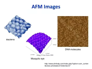
Explore the latest advances in Atomic Force Microscopy (AFM) imaging and force modes using Worm-Like Chain (WLC) models for studying proteins and DNA. Learn how to optimize imaging to minimize noise and use different AFM operating modes effectively.

AFM II
E N D
Presentation Transcript
Imaging Mode: don’t be at zero frequency (because of Noise) Force Mode: Worm-Like Chain (WLC): very good for proteins and DNA. AFM AFM II
(Back to) AFM Imaging Mode. • To minimize noise, go to a higher frequency : noise always goes like 1/f (f = frequency) Force Mode. • Force Mode: Worm Like Chain model of Protein Folding (and DNA)
AFM—Imaging Mode(s) Force – one place Imaging – Scan Ionic repulsion, bends tip Measure (z-axis) distance, Or Constant force (by altering distance with feedback) Muller, Biochemistry, 2008 http://cp.literature.agilent.com/litweb/pdf/5990-3293EN.pdf http://www.home.agilent.com/agilent/editorial.jspx?cc=US&lc=eng&ckey=1774141&nid=-33986.0.02&id=1774141
Operating Modes of AFM The most commonly used modes of operation of an AFM are: 1. Contact mode AFM (aka C-AFM or CMAFM) 2. Tapping mode AFM (aka TMAFM, IC-AFM or AM-AFM) 3. Noncontact mode (aka NC-AFM, close contact AFM or FM-AFM). (Lots of different names because of patent squabbles!) Contact is often called a static mode, and Tapping and noncontact called dynamic modes, as the cantilever is oscillated in Tapping and noncontact modes. Typically this is done by adding an extra piezoelectric element that oscillates up and down at somewhere between 5-400kHz to the cantilever holder. http://www.afmhelp.com/index.php option=com_content&view=article&id=51&Itemid=57
The main difference between tapping mode and noncontact mode In tapping mode, the tip of the probe actually touches the sample, and moves completely away from the sample in each oscillation cycle. In NC-AFM, the cantilever stays close to the sample all the times, and has a much smaller oscillation amplitude. NC-AFM (noncontact AFM) is more sensitive to small oscillations of the cantilever, so may be operated in close contact (almost touching). Noncontact AFM, unlike the other AFM techniques can obtain true atomic resolution images. AM-AFM, typically used for Tapping mode – where the tip actually taps the sample during each oscillation. This is often the most stable mode to use in air, and so is currently more commonly used than either noncontact or contact modes for most applications. By detecting at non-zero frequency, the noise is often less! http://www.afmhelp.com/index.php?option=com_content&view=article&id=51&Itemid=57
1/f noise is ubiquitous! If you can measure at non-zero frequency, often due better! Very Common Fig: The plot of the power spectral density S(f) vs. frequency f for a full open state at . A power law , , fits the data quite well. http://www.scholarpedia.org/article/1/f_noise Stay away from DC measurements (when possible) http://iopscience.iop.org/0295-5075/73/3/457/fulltext/epl9165.html
AFM— Force Modes Force – one place http://cp.literature.agilent.com/litweb/pdf/5990-3293EN.pdf http://www.home.agilent.com/agilent/editorial.jspx?cc=US&lc=eng&ckey=1774141&nid=-33986.0.02&id=1774141
Simply Hookian Spring doesn’t fit data well F= - kx Hooke’s Law: You apply a force on something and it increases in length linearly. Proportional constant = k. Minus sign because it’s a restoring force. What does F vs. x look like for a (Hookian) Spring? There’s a lot of entropy which takes energy to straighten (zero) out. DNA is much longer than it is wide – λ DNA (virus DNA) is about 16.5 µm upon full extension, but the molecule’s diameter is only about 2 nanometers, or some four orders of magnitude smaller. Can expect some simplification where don’t need to get into details of molecular bonding. Like liquids– need to know mass density (r), viscosity (h)—forget about details. http://biocurious.com/2006/07/04/wormlike-chains
Two Models of DNA • (simple) Freely Jointed Chain (FJC) • 2. (more complicated) Worm-like Chain (WLC) Idealized FJC: FJC: Head in one direction for length b, then turn in any direction for length b. [b= Kuhn length = ½ P, where P= Persistence Length] At small z, gives F= -kz. It isn’t a bad fit for ssDNA, where each individual non-paired base acts as an individual segment, but it fails miserably at high forces for dsDNA. FJC: Completely straight, unstretchable. No thermal fluctuations away from straight line are allowed The polymer can only disorder at the joints between segments FJC: Can think of DNA as a random walk in 3-D.
Force vs. Extension for DNA F=-kx works well at very low force; at higher force, DNA is extended (> 50%), need FJC; or better is WLC At very low (< 100 fN) and at high forces (> 5 pN), the FJC does a good job. In between it has a problem. There you have to use WJC. You measure the Persistence length Strick, J. Stat. Physics,1998.
Two Models of DNA 1. (simple) Freely Jointed Chain (FJC) 2. (more complicated) Worm-like Chain (WLC) Realistic Chain: WLC: Have a correlation or persistence length (= Lp). The force extension curve [F(x) versus x is well described by the WLC equation Where Lp: persistence length, a measure of the chains bending rigidity = 2x Kuhn Length L = contour length z = extension
WLC Fits very well at most stretches For DNA The force extension curve [F(x) versus x is well described by the WLC equation WLC works well for DNA and Proteins
WLC for DNA beyond 20 pN What’s happening at forces > 20 pN? The above fit is good to about 10-15 pN, above which the model keeps increasing quicker than the experimental data. This is because the WLC model is an inextensible model, where the chain contour length is constant2. Further modifications to the wormlike chain have introduced an enthalpic correction for higher forces, where the applied force is no longer simply extending the molecule, but has started doing work on the structure itself, deforming it from its regular B-DNA form. This addition makes the model valid up to approximately 60 pN, at which point DNA undergoes a structural phase transition and the force-extension relation changes quite rapidly back to a more Hookean form, extending up to 1.6x its normal contour length before displaying further non-linearities. http://biocurious.com/2006/07/04/wormlike-chains
Titin: Human’s Biggest protein Silicon Nitride lever: 10’s pN – several nN’s measureable Each domain IgG Titin: 4.2MDa; Gene (on # 2) = 38,138 aa: Goes from Z-disk to Center; stretchy =I Band Cardiac (N2B &N2BA), Skeletal (N2A), Smooth all have different regions.
Reversible Unfolding by AFM Pulling on Titin Simple model: Upon reaching a certain force (peaks), the abrupt unfolding of a domain lengthens the polypeptide by 28 to 29 nm and reduces the force (troughs) to that of the value predicted by the force extension curve of the enlarged polypeptide. Gold Reversible Unfolding of Individual Titin Immunoglobulin Domains by AFM, Science, M. Reif, H. Gaub, 1997
Nontopographic modes of AFM Apart from the topographic modes that collect images, there are many modes designed to measure other properties of the sample. For example: Magnetic Force Microscopy, MFM, measures the distribution of magnetic field in the sample. Kelvin Probe Microscopy (KPM) measures contact potential difference across the sample. Force Spectroscopy can measure individual molecular interactions. Nanoindentation can measure hardness or softness of the sample. Thermal modes can measure thermal parameters, for example, thermal conductivity on the nanoscale. http://www.afmhelp.com/index.php?option=com_content&view=article&id=51&Itemid=57
Obtaining the Tip Geometry For studying the tip influence on the data we need to know tip geometry first. In general, the geometry of the SPM tip can be determined in these ways: 1. use manufacturer's specifications (tip geometry, apex radius and angle) 2. use scanning electron microscope of other independent technique to determine tip properties 3. use known tip characterizer sample (with steep edges) 4. use blind tip estimation algorithm together with tip characterizers or other suitable samples http://gwyddion.net/documentation/user-guide-en/tip-convolution-artefacts.html