Flow Analysis
Flow Analysis. Factors that Affect the Flow Pattern Flow Analysis Information Flow Patterns a. Flow within Workstations b. Flow within Departments c. Flow between Departments Flow Planning Measuring Flow Types of Layout a. Fixed Location b. Product c. Group Technology d. Process

Flow Analysis
E N D
Presentation Transcript
Flow Analysis • Factors that Affect the Flow Pattern • Flow Analysis Information • Flow Patterns a. Flow within Workstations b. Flow within Departments c. Flow between Departments • Flow Planning • Measuring Flow • Types of Layout a. Fixed Location b. Product c. Group Technology d. Process e. Hybrid • Flow Dominance Measure • Techniques for Machine Cell Formation a. Row and Column Masking Algorithm b. Single Linkage Clustering c. Average Linkage clustering
Factors that Affect the Flow Pattern • Number of parts in each product • Number of operations on each part • Sequence of operations in each part • Number of subassemblies • Number of units to be produced • Product versus process type layout • Desired flexibility • Locations of service areas • The building • . . . .
Flow Analysis Information • Assembly Chart • Operations Process Chart • Flow Process Chart • Multi-Product Process Chart • Flow Diagram • From-To Chart
Assembly Chart It is an analog model of the assembly process. Circles with a single link denote basic components, circles with several links denote assembly operations/subassemblies, and squares represent inspection operations. The easiest method to constructing an assembly chart is to begin with the original product and to trace the product disassembly back to its basic components.
Operations Process Chart By superimposing the route sheets and the assembly chart, a chart results that gives an overview of the flow within the facility. This chart is operations process chart.
Flow Process Chart This chart uses circles for operations, arrows for transports, squares for inspections, triangles for storage, and the letter D for delays. Vertical lines connect these symbols in the sequence they are performed.
Multi-Product Process Chart This chart is a flow process chart containing several products.
Flow Diagram It depicts the probable movement of materials in the floor plant. The movement is represented by a line in the plant drawing.
From-To Chart This chart is a matrix that contains numbers representing a measure (units, unit loads, etc.) of the material flow between machines, departments, buildings, etc.
Flow Patterns: Flow within Workstations Motion studies and ergonomics considerations are important in establishing the flow within workstations. Flow within workstations should be: • Simultaneous: coordinated use of hands, arms and feet. • Symmetrical: coordination of movements about the center of the body. • Natural: movements are continuous, curved, and make use of momentum. • Rhythmical and Habitual: flow allows a methodological and automatic sequence of activities. It should reduce mental, eye and muscle fatigue, and strain.
Flow Patterns: Flow within Departments • The flow pattern within departments depends on the type of department. • In a product and/or product family department, the flow follows the product flow. 2 machines/operator 1 machine/operator 1 machine/operator END-TO-END BACK-TO-BACK FRONT-TO-FRONT More than 2 machines /operator 1 machine/operator CIRCULAR ODD-ANGLE
One way Aisle Aisle Aisle Aisle Aisle One way Flow Pat.: Flow within Departments (cont.) • In a process department, little flow should occur between workstations within departments. Flow occurs between workstations and isles. Uncommon DIAGONAL PARALLEL PERPENDICULAR Dependent on interactions among workstations available space size of materials
Flow Pat.: Flow between Departments • Flow between departments is a criterion often used to evaluate flow within a facility. • Flow typically is a combination of the basic horizontal flow patterns shown below. An important consideration in combining the flow patterns is the location of the entrance (receiving department) and exit (shipping department). Similar to straight. It is not as long. L flow Simplest. Separate receiving/shipping crews Straight Very popular. Combine receiving /shipping. Simple to administer Circular flow U flow Terminate flow. Near point of origin Serpentine When line is too long S flow
Flow within a facility considering the locations of entrance and exit At the same location On adjacent sides
Flow within a facility considering the locations of entrance and exit (cont.) On the same side but at opposite ends On opposite sides
Vertical Flow Pattern Flow between buildings exists and the connection between buildings is elevated Ground level ingress (entry) and egress (exit) occur on the same side of the building Ground level ingress (entry) and egress (exit) are required Some bucket and belt conveyors and escalators result in inclined flow Travel between floors occurs on the same side of the building Backtracking occurs due to the return to the top floor
Flow Planning • Planning effective flow involves combining the above patterns with adequate isles to obtain progressive movements from origin to destination. • An effective flow can be achieved by maximizing directed flow paths, reducing flow, and minimizing the costs of flow. • A directed flow path is an uninterrupted flow path progressing directly from origin to destination: the figure below illustrates the congestion and undesirable intersections that may occur when flow paths are interrupted. Uninterrupted flow paths Interrupted flow paths
Flow Planning (cont.) • The reduction of flow can be achieved by work simplification including: 1. Eliminating flow by planning for the delivery of materials, information, or people directly to the point of ultimate use and eliminate intermediate steps. 2. Minimizing multiple flows by planning for the flow between two consecutive points of use to take place in as few movements as possible. 3. Combining flows and operations whenever possible by planning for the movement of materials, information, or people to be combined with a processing step. • Minimizing the cost of flow can be achieved as follows: 1. Reduction of manual handling by minimizing walking, manual travel distances, and motions. 2. Elimination of manual handling by mechanizing or automating flow.
Measuring Flow 1. Flow among departments is one of the most important factors in the arrangement of departments within a facility. 2. Flows may be specified in a quantitative manner or a qualitative manner. Quantitative measures may include pieces per hour, moves per day, pounds per week. Qualitative measures may range from an absolute necessity that two departments show be close to each other to a preference that two departments not being close to each other. 3. In facilities having large volumes of materials, information, a number of people moving between departments, a quantitative measure of flow will typically be the basis for the arrangement of departments. On the contrary, in facilities having very little actual movement of materials, information, and people flowing between departments, but having significant communication and organizational interrelation, a qualitative measure of flow will typically serve as the basis for the arrangement of departments. 4. Most often, a facility will have a need for both quantitative and qualitative measures of flow and both measures should be used. 5. Quantitative flow measure: From-to Chart Qualitative flow measure: Relationship (REL) Chart
Quantitative Flow Measurement • A From-to Chart is constructed as follows: 1. List all departments down the row and across the column following the overall flow pattern. 2. Establish a measure of flow for the facility that accurately indicates equivalent flow volumes. If the items moved are equivalent with respect to ease of movement, the number of trips may be recorded in the from-to chart. If the items moved vary in size, weight, value, risk of damage, shape, and so on, then equivalent items may be established so that the quantities recorded in the from-to chart represent the proper relationships among the volumes of movement. 3. Based on the flow paths for the items to be moved and the established measure of flow, record the flow volumes in the from-to chart.
Stores Milling Turning Press Plate Assembly Warehouse Stores Turning Milling Press Plate Assembly Warehouse –126914 – ––––72 – –3––4– – –– ––31 1 –31––4 3 1– –––– 7 –––––– – Stores Milling Turning Press Plate Assembly Warehouse –612914 – ––3–4– – ––––72 – –– ––31 1 –13––4 3 1– –––– 7 –––––– – Stores Turning Milling Press Plate Assembly Warehouse Example 1 From-to Chart Revised Flow Pattern Original Flow Pattern
Flow Patterns Press Turning Milling Store Plate Press Assembly Warehouse Stores Turning Milling Warehouse Assembly Plate U-shaped flow Straight-line flow Stores Press Plate Assembly Turning Milling Warehouse Stores Milling Warehouse Turning Press Plate Assembly S-shaped flow W-shaped flow
Flow Patterns (cont.) Press Turning Milling Store Plate Press Assembly Warehouse Stores Turning Milling Warehouse Assembly Plate U-shaped flow Straight-line flow Stores Press Plate Assembly Turning Milling Warehouse Stores Milling Warehouse Turning Press Plate Assembly S-shaped flow W-shaped flow
Qualitative Flow Measurement • A Relationship (REL) Chart is constructed as follows: 1. List all departments on the relationship chart. 2. Conduct interviews of surveys with persons from each department listed on the relationship chart and with the management responsible for all departments. 3. Define the criteria for assigning closeness relationships and itemize and record the criteria as the reasons for relationship values on the relationship chart. 4. Establish the relationship value and the reason for the value for all pairs of departments. 5. Allow everyone having input to the development of the relationship chart to have an opportunity to evaluate and discuss changes in the chart.
Code Reason 1 Frequency of use high 2 Frequency of use medium 3 Frequency of use low 4 Information flow high 5 Information flow medium 6 Information flow low 1. Directors conference room 2. President 3. Sales department 4. Personnel 5. Plant manager 6. Plant engineering office 7. Production supervisor 8. Controller office 9. Purchasing department I 1 O 5 U 6 O 5 A 4 I 4 U 6 I 4 I 1 U 6 I 4 O 5 A 4 O 5 O5 U 3 O 5 O 5 O 5 O 5 E 4 O 2 U 6 O 5 O 5 O 5 U 3 U 6 E 4 O 4 U 3 I 4 I 4 U 3 O 5 U 6 Rating Definition A Absolutely Necessary E Especially Important I Important O Ordinary Closeness OK U Unimportant X Undesirable Relationship Chart
Types of Layout Volume High Medium Low Product Planning Department Product Layout Product Family Planning Department Fixed Location Layout Process Layout Group Technology Layout Fixed Materials Location Planning Department Process Planning Department Low Medium High Variety
Lathe Press Grind Weld Assembly Paint Fixed Product Layout Warehouse Storage
Fixed Product Layout (cont.) • Advantages 1. Material movement is reduced. 2. Promotes job enlargement by allowing individuals or teams to perform the “whole job”. 3. Continuity of operations and responsibility results from team. 4. Highly flexible; can accommodate changes in product design, product mix, and product volume. 5. Independence of production centers allowing scheduling to achieve minimum total production time. • Limitations 1. Increased movement of personnel and equipment. 2. Equipment duplication may occur. 3. Higher skill requirements for personnel. 4. General supervision required. 5. Cumbersome and costly positioning of material and machinery. 6. Low equipment utilization.
Warehouse Assembly Drill Grind Drill Lathe Drill Drill Lathe Bend Lathe Mill Press Drill Storage Product Layout
Product Layout (cont.) • Advantages 1. Since the layout corresponds to the sequence of operations, smooth and logical flow lines result. 2. Since the work from one process is fed directly into the next, small in-process inventories result. 3. Total production time per unit is short. 4. Since the machines are located so as to minimize distances between consecutive operations, material handling is reduced. 5. Little skill is usually required by operators at the production line; hence, training is simple, short, and inexpensive. 6. Simple production planning control systems are possible. 7. Less space is occupied by work in transit and for temporary storage. • Limitations 1. A breakdown of one machine may lead to a complete stoppage of the line that follows that machine. 2. Since the layout is determined by the product, a change in product design may require major alternations in the layout. 3. The “pace” of production is determined by the slowest machine. 4. Supervision is general, rather than specialized. 5. Comparatively high investment is required, as identical machines (a few not fully utilized) are sometimes distributed along the line.
Warehouse Paint Lathe Drill Weld Mill Drill Grind Lathe Weld Mill Lathe Mill Paint Grind Assembly Assembly Lathe Mill Storage Process Layout
Process Layout (cont.) • Advantages 1. Better utilization of machines can result; consequently, fewer machines are required. 2. A high degree of flexibility exists relative to equipment or man power allocation for specific tasks. 3. Comparatively low investment in machines is required. 4. The diversity of tasks offers a more interesting and satisfying occupation for the operator. 5. Specialized supervision is possible. • Limitations 1. Since longer flow lines usually exist, material handling is more expensive. 2. Production planning and control systems are more involved. 3. Total production time is usually longer. 4. Comparatively large amounts of in-process inventory result. 5. Space and capital are tied up by work in process. 6. Because of the diversity of the jobs in specialized departments, higher grades of skill are required.
Warehouse Grind Drill Grind Assembly Drill Weld Assembly Lathe Assembly Press Mill Lathe Paint Drill Drill Press Assembly Grind Storage Group Layout
Group Layout (cont.) • Advantages 1. Increased machine utilization. 2. Team attitude and job enlargement tend to occur. 3. Compromise between product layout and process layout, with associated advantages. 4. Supports the use of general purpose equipment. 5. Shorter travel distances and smoother flow lines than for process layout. • Limitations 1. General supervision required. 2. Higher skill levels required of employees than for product layout. 3. Compromise between product layout and process layout, with associated limitations. 4. Depends on balanced material flow through the cell; otherwise, buffers and work-in-process storage are required. 5. Lower machine utilization than for process layout.
DM TM TM TM TM TM BM Hybrid Layout • Combination of the layouts discussed. • A sample hybrid layout that has characteristics of group, process and product layout is shown in the following figure. • A combination of group layout in manufacturing cells, product layout in assembly area, and process layout in the general machining and finishing section is used.
Flow Dominance Measure • Notations: M: number of activities. Nij: number of different types of items moved between activities i and j. fijk: flow volume between i and j for item k (in moves/time period). hijk: equivalence factor for moving item k with respect to other items moved between i and j (dimensionless). wij: equivalent flow volume specified in from-to chart (in moves/time period),
Flow Dominance Measure (cont.) • Flow dominance measure = f = where • f is the coefficient of variation. • fL and fU are lower and upper bounds on f, respectively (fL f fU). • The upper bound fU is only guaranteed to work when each process plan includes all activities. In this case, 0 f 1.
Flow Dominance Measure (cont.) Three cases : 1. f 0 a few dominant flows exist. product layout. can use operations process chart as starting point for developing layout and material handling system design. quantitative measures principal source of activity relationship. 2. f 1 many nearly equal flows exist. any layout equally good with respect to flows . qualitative measures principal source of activity relationship. 3. 0 << f << 1 no dominant flows exist. difficult to develop layout. process or product family layout . both quantitative and qualitative measures important source of activity relationship.
Example 2 • Given three machines (activities) labeled 1, 2 & 3, Product A B C Process Plan 1 - 2 - 3 2 - 1 3 - 1 - 2 Quantities/Shift 10 5 15 • Assume Product B is twice as “difficult” to move as A or C hijB = 2 and hijA = hijC = 1 To 1 0 2 5 10 1 15 15 2 110 1 15 25 0 0 3 0 1 10 10 0 From 1 2 3 Equivalent Flow Volume From-To Chart w12 = 25, w21 = 10, etc
Example 2 (cont.) M = 3 and no dominant flows exist (likely, since 3 different process plans)
Qualitative Measures • Closeness values (A, E, I, O, U, X) used to indicate physical proximity requirements between activities. • Relationship Chart can only show symmetric relationships, as compared to From-to Chart (wij wji possible). • Relationship Chart is starting point for developing layout when 0 << f 1. • If f 1, then don’t need to consider flow (only qualitative relationship) • If f <<1, then one can convert equivalent flow volumes to closeness values so that material flow relationships can be considered along with qualitative relationship. • If f 0, then can still convert to relationship chart if significant qualitative relationship exists, otherwise, just use operations process chart.
A I E Machine 1 Machine 2 Machine 3 Conversion Method • To convert equivalent flow volumes to closeness values for the example problem, use wij + wji to make them symmetric. • Conversion relations : 20 < wij + wji A w12 + w21 = 25 + 10 A 12 < wij + wji 20 E w13 + w31 = 0 + 15 E 5 < wij + wji 12 I w23 + w32 = 10 + 0 I 0 < wij + wji 5 O wij + wji = 0 U
Group Technology • Group Technology (GT) is a management philosophy that attempts to group products with similar design or manufacturing characteristics, or both. • Cellular Manufacturing (CM) is an application of GT that involves grouping machines based on the parts manufactured by them. • The main objective of CM is to identify machine cells and part families simultaneously, and to allocate part families to machine cells in a way that minimizes the intercellular movement of parts. • Potential benefits of CM: * Setup time reduction. * Improvement in quality. * Work-in-process (WIP) reduction. * Improvement in material flow. * Material handling cost reduction. * Improvement in machine utilization. * Direct/indirect labor cost reduction. * Improvement in space utilization. * Improvement in employee moral.
Group Technology (cont.) • A cellular manufacturing system (CMS) designer must consider a number of constraints: • Available capacity of machines in each cell cannot be exceeded. • Safety and technological requirements pertaining to the location of equipment and processes must be met. • The size of a cell and the number of cells must not exceed a user-specified value. • Design analysis begins with a machine-part indicator matrix A = [aij] of size m×n, where m is the number of machines and n the number of parts. Typically the matrix consists of 0 and 1 entries: • aij = 1 indicates that part j is processed by machine i. • aij = 0 indicates that part j is not processed by machine i. • Analysis attempt to rearrange the rows and columns of the matrix to get a block diagonal form as shown in the following example.
Initial Machine Part Processing Matrix Rearranged Machine-Part Processing Matrix Part Part P1 P2 P3 P4 P5 P6 P1 P3 P2 P4 P5 P6 1––––– –1–1–1 –1–11– 1– 1––– –1–––1 1–1––– ––––11 1––––– 11–––– 11–––– –– 11–1 ––111– ––1––1 ––––11 M1 M2 M3 M4 M5 M6 M7 M1 M4 M6 M2 M3 M5 M7 Machine Machine Example 3
Row and Column Masking (R&CM) Algorithm 1. Draw a horizontal line through the first row. Select any 1 entry in the matrix through which there is only one line. 2. If the entry has a horizontal line, go to step 2a. If the entry has a vertical line, go to step 2b. 2a. Draw a vertical line through the column in which this 1 entry appears. Go to step 3. 2b. Draw a horizontal line through the row in which this 1 entry appears. Go to step 3. 3. If there is any 1 entries with only one line through them, select any one and go to step 2. Repeat until there are no such entries left. Identify the corresponding machine cell and part family. Go to step 4. 4. Select any row through which there is no line. If there are no such rows, stop. Otherwise, draw a horizontal line through this row, select any 1 entry in the matrix through which there is only one line, and go to step 2.
Identification of the First Machine Cell and Part Family Identification of the Second Machine Cell and Part Family Part Part P1 P2 P3 P4 P5 P6 P1 P2 P3 P4 P5 P6 2 3 4 2 3 4 7 1––––– –1–1–1 –1–11– 1– 1––– –1–––1 1–1––– ––––11 M1 M2 M3 M4 M5 M6 M7 1––––– –1–1–1 –1–11– 1– 1––– –1–––1 1–1––– ––––11 M1 M2 M3 M4 M5 M6 M7 Machine Machine 15 8 6 15 Example 3 Solution
Single Linkage (S-Link) Clustering Algorithm • S-Link is the simplest of all clustering algorithms based on the similarity coefficient method. • The similarity coefficient between two machines is defined as the number of parts visiting the two machines divided by the number of parts visiting either of the two machines. 1. pairwise similarity coefficients between machines are calculated and stored in the similarity matrix. 2. The two most similar machines join to form the first machine cell. 3. The threshold value (the similarity level at which two or more machine cells join together) is lowered in predetermined steps and all machine/machine cells with the similarity coefficient greater than the threshold value are grouped into larger cells. 4. Step 3 is repeated until all machines are grouped into a single machine cell.
Part P1 P2 P3 P4 P5 P6 P7 P8 P9 P10 P11 P12 P13 P14 P15 P16 P17 P18 P19 P20 P21 P22 M1 M2 M3 M4 M5 M6 M7 M8 M9 M10 M11 1 1 1 – – – – – – – 1 – – – 1 1 – – – 1 1 1 – – – – 1 – – 1 – – 1 1 – – – – – – 1 – – – – – – – 1 1 – – – – – 1 1 – – – – – 1 – – – 1 1 1 – – – – – – – 1 – – – 1 1 – – – 1 1 1 1 1 1 – – – 1 – – – – – – – 1 1 – – – 1 1 1 – – – – 1 – – 1 – – – 1 – – – – – – 1 – – – – – – 1 – 1 – – 1 – – – – 1 – – 1 1 – – – – – – – – 1 1 – – 1 1 – 1 1 1 – – 1 1 1 – – – – – – 1 – – – – 1 – – – – 1 – – 1 1 – – – – 1 1 1 – 1 – 1 1 – – 1 1 – – 1 – – – – – – – – – – 1 – – – – 1 1 – – – – – – 1 1 – – – – Machine Example 4: Initial Machine Part Matrix
Example 4: Initial Similarity Coefficient Matrix Machine M1 M2 M3 M4 M5 M6 M7 M8 M9 M10 M11 M1 M2 M3 M4 M5 M6 M7 M8 M9 M10 M11 – 0.08– 0.000.43– 1.000.08 0.00– 0.800.000.000.80– 0.000.800.500.000.00– 0.000.000.100.000.000.00– 0.000.250.500.000.000.270.45– 0.000.000.000.000.000.000.830.36– 0.430.450.230.430.430.360.000.170.00– 0.000.000.000.000.000.000.570.370.670.00– Machine