Download

1 / 37
370 likes | 492 Vues
This presentation elaborates on the concept of Set Similarity Join (SSJoin) at Penn State University, discussing both approximate and exact methods. It highlights the significance of weighting tokens to express their relative importance during join operations. The session covers various applications, such as entity resolution and movie recommendations, while addressing challenges like scalability and efficiency in SQL expressions. Additionally, it explores diverse similarity functions and introduces techniques like blocking and inverted indexing for enhancing performance.

E N D
Weighted Exact Set Similarity Join The Pennsylvania State University Dongwon Lee dongwon@psu.edu
Set Similarity Join • Def. Set Similarity Join (SSJoin): Between collections A and B, find X pairs of objects whose similarity > t: • If X = “MOST” Approximate SSJoin • If X = “ALL” Exact SSJoin 0.7 : {Lake, Monona, Wisc, Dane, County} 0.5 0.4 : {University, Mendota, Wisc, Dane,} 0.2 0.9 0.1 A B Wisconsin DB Seminar, 2009
Set Similarity Join • Weighted vs. Unweighted • Weighting quantifies relative importance of token • Eg, “Microsoft” is more important than “Copr.” • How to assign meaningful weights to tokens is an important problem itself • Not further discussed here Wisconsin DB Seminar, 2009
Set Similarity Join • Approximate SSJoin • Allows some false positives/negatives • Eg, LSH as solution • Exact SSJoin • Does not allow any false positives/negatives • Needs to be scalable • Weighted + Exact SSJoin • Will simply call “WESSJoin” UESSJoin WESSJoin exact UASSJoin WASSJoin approx. unweighted weighted Wisconsin DB Seminar, 2009
Applications of WESSJoin • Entity resolution • Web document genre classification • Find all pairs of documents w. similar contents • Query refinement for web search • For a query, find another w. similar search result • Movie recommendation • Identify users who have similar movie tastes w.r.t. the rented movies Focus on string data represented as SET • Eg, document, web page, record Wisconsin DB Seminar, 2009
Research Issues • Why not express WESSJoin in SQL? • Join predicate as UDF • Cartesian product followed by UDF processing Inefficient evaluation • Special handling for WESSJoin needed • Scalability • Support diverse similarity (or distance) functions • Eg, Overlap, Jaccard, Cosine vs. Edit, … • Support diverse computation models • Eg, Threshold vs. Top-k Wisconsin DB Seminar, 2009
Similarity/Distance Functions • Jaccard Coefficient: J(x,y) = • Overlap similarity: O(x,y) = • Cosine similarity: C(x,y) = • Hamming distance H(x,y) = • Levenshtein distance L(x,y): min # of edit operations to transform x to y Wisconsin DB Seminar, 2009
Properties of sim() • Similarity functions can be re-written to each other equivalently • J(x,y) > t O(x,y) > t/(1+t) (|x|+|y|) • O(x,y) > t H(x,y) < |x|+|y|-2t • C(x,y) > t O(x,y) > • Eg, • x: {Lake, Mendota, Monona} • y: {Wisc, Dane, Mendota, Lake} • J(x,y) > 0.5 ? O(x,y) > 2.3 ? • Set representation: k-gram, word, phrase, … Wisconsin DB Seminar, 2009
Naïve Solution • All pair-wise comparison between A and B • Nested-loop: |A||B| comparisons • The sim() evaluation may be costly • Eg, Generalized Jaccard Similarity function with O(|x|3) For x in A: For y in B: If sim(x,y) > t, return (x,y); A, B: table x, y: record as set Wisconsin DB Seminar, 2009
Naïve Solution Example A B O(x,y) > 2 ? Wisconsin DB Seminar, 2009
Naïve Solution Example A B J(x,y) > 0.6 ? Wisconsin DB Seminar, 2009
2-Step Framework • Step 1: “Blocking” • Using Index/heuristics/filtering/etc, reduce # of candidates to compare • Step 2: sim() only within candidate sets • O(|A||C|) s.t. |C| << |B| For x in A: Using Foo, find a candidate set C in B For y in C: If sim(x,y) > t, return (x,y); Wisconsin DB Seminar, 2009
Variants for “Foo” • “Foo”: How to identify candidate set C • Fast • Accurate: no false positives/negatives • Many Variants for “Foo” • Inverted Index [Sarawagi et al, SIGMOD 04] • Size filtering [Arasu et al, VLDB 06] • Prefix Index [Chaudhuri et al, ICDE 06] • Prefix + Inverted Index [Bayardo et al, WWW 07] • Bound filtering [On et al, ICDE 07] • Position Index [Xiao et al, WWW 08] Wisconsin DB Seminar, 2009
Inverted Index [Sarawagi et al, SIGMOD 04] A B Inverted Index (IDX) for A Inverted Index (IDX) for B Wisconsin DB Seminar, 2009
Inverted Index [Sarawagi et al, SIGMOD 04] A B Inverted Index (IDX) for B For x in A: Using IDX, find a candidate set C in B For y in C: If sim(x,y) > t, return (x,y); ID=1: {Lake, Mendota} ID=2: … ID=3: … Candidate set C: {4,6} + {6} = {4, 6} Wisconsin DB Seminar, 2009
Inverted Index [Sarawagi et al, SIGMOD 04] A B Inverted Index (IDX) for B For x in A: Using IDX, find a candidate set C in B For y in C: If sim(x,y) > t, return (x,y); ID=1: {Lake, Mendota} ID=2: … ID=3: … Candidate set C: O(x,y) > 2 Wisconsin DB Seminar, 2009
Size Filtering [Arasu et al, VLDB 06] • Idea: Build index on the size of inputs • Jaccard Coefficient J= • Upperbound for Jaccard: • Bounding |y| w.r.t. |x|: • Combining two x x y y Wisconsin DB Seminar, 2009
Size Filtering [Arasu et al, VLDB 06] • Intuition: If t and |x| are given, |y| is bounded • Eg, • x: {Lake, Mendota} • y: {Lake, Mendota, Monona, Area} • J(x,y) > 0.8 ? • Then, according to: • |x|=2, t=0.8 1.6 <= |y| <= 2.5 • However, |y| = 4 • y cannot satisfy t=0.8 no need to compute J(x,y) at all Wisconsin DB Seminar, 2009
Size Filtering [Arasu et al, VLDB 06] • Algorithm • For all input strings, build B-tree w.r.t. their sizes • Given a set x, using B-tree index, find a candidate y in B s.t. For x in A: Using IDX, find a candidate set C in B For y in C: If sim(x,y) > t, return (x,y); Wisconsin DB Seminar, 2009
Prefix Index [Chaudhuri et al, ICDE 06] • Intuition: If two sets are very similar, their prefixes, when ordered, must have some common tokens • Eg. • x: {Dane, University, Monona, Mendota} • y: {Area, Lake, Mendota, Monona, Wisc} • O(x,y) > 3 ? • x’: {Dane, Mendota, Monona, University} • y’: {Area, Lake, Mendota, Monona, Wisc} Prefixes Wisconsin DB Seminar, 2009
Prefix Index [Chaudhuri et al, ICDE 06] Theorem 1: If there is no overlap btw. Prefix(x) and Prefix(y), then sim(x,y) > t, where: • If sim()=Overlap, Prefix(x)=|x| - (t-1) • If sim()=Jaccard, Prefix(x)=|x|-Ceiling(t*|x|)+1 • Algorithm using Theorem 1: • Given a set x • For each token t_x in the prefix of x • Using an index, locate a candidate y that contains t_x in the prefix of y • If sim(x,y) > t, return (x,y) Wisconsin DB Seminar, 2009
Prefix + Inverted Index[Bayardo et al, WWW 07] A B Inverted Index (IDX) for both A and B Create a universal order: Put rare tokens front Order: Dane > Research > University > Area > Mendota > Lake > Monona Wisconsin DB Seminar, 2009
Prefix + Inverted Index[Bayardo et al, WWW 07] Ordered A Ordered B Order: Dane > Research > University > Area > Mendota > Lake > Monona Wisconsin DB Seminar, 2009
Prefix + Inverted Index[Bayardo et al, WWW 07] Ordered A Ordered B O(x,y) > 2 Prefix(x)=|x|-(t-1)=|x|-1 Prefix Inverted Index for B ID=1: {Mendota, Lake} ID=2: … ID=3: … Candidate set C: {6} Wisconsin DB Seminar, 2009
Prefix + Inverted Index[Bayardo et al, WWW 07] Ordered A Ordered B O(x,y) > 2 Prefix(x)=|x|-(t-1)=|x|-1 Prefix Inverted Index for B ID=1: … ID=2: {Area, Lake, Monona} ID=3: … Candidate set C: {5} + {4,6} = {4,5,6} Wisconsin DB Seminar, 2009
Prefix + Inverted Index[Bayardo et al, WWW 07] Ordered A Ordered B O(x,y) > 2 Prefix(x)=|x|-(t-1)=|x|-1 Prefix Inverted Index for B ID=1: … ID=2: … ID=3: {Dane, Mendota, Lake, Monona} Candidate set C: {6} + {4,6} = {4,6} Wisconsin DB Seminar, 2009
Position Index [Xiao et al, WWW 08] Order: Dane > Research > University > Area > Mendota > Lake > Monona • Eg, • x: {Dane, Research, Area, Mendota, Lake} • y: {Research, Area, Mendota, Lake, Monona} • O(x,y) > 4 ? • • Prefix(x) = Prefix(y) = 5 – (4 -1) = 2 • x: {Dane, Research, Area, Mendota, Lake} • y: {Research, Area, Mendota, Lake, Monona} • “Research” is common btw prefixes (x,y) is a candidate pair need to compute sim(x,y) Wisconsin DB Seminar, 2009
Position Index [Xiao et al, WWW 08] Order: Dane > Research > University > Area > Mendota > Lake > Monona • Eg, • x: {Dane, Research, Area, Mendota, Lake} • y: {Research, Area, Mendota, Lake, Monona} • O(x,y) > 4 ? • • Prefix(x) = Prefix(y) = 5 – (4 -1) = 2 • x: {Dane, Research, Area, Mendota, Lake} • y: {Research, Area, Mendota, Lake, Monona} • Estimation of max overlap = overlap in prefixes + min # of unseen tokens = 1 + min(3,4) = 4 > t No need to compute sim(x,y) ! Wisconsin DB Seminar, 2009
Bound Filtering [On et al, ICDE 07] • Generalized Jaccard (GJ) similarity • Two sets: x = {a1, …, a|x|}, y = {b1, …, b|y|} • Normalized weight of the maximum bipartite matching M in the bipartite graph (N = x U y, E=x X y) Wisconsin DB Seminar, 2009
x y Bound Filtering [On et al, ICDE 07] 0.7 0.7 0.5 0.5 0.4 0.4 0.2 0.9 0.2 0.9 0.1 0.1 x y M: maximum weight bipartite matching Wisconsin DB Seminar, 2009
Bound Filtering [On et al, ICDE 07] • Issues • GJ captures more semantics btw. two sets via the weighted bipartite matching than Jaccard • But more costly to compute: maximum weight bipartite matching • Bellman-Ford: O(V2E) • Hungarian: O(V3) For x in A: Using Foo, find a candidate set C in B For y in C: If GJ(x,y) > t, return (x,y); Wisconsin DB Seminar, 2009
Bound Filtering [On et al, ICDE 07] • Bipartite matching computation is expensive because of the requirement • No node in the bipartite graph can have more than one edge incident on it • Relax this constraint: • For each element aiin x, find an element bj in y with the highest element-level similarity S1 • For each element bjin y, find an element ai in x with the highest element-level similarity S2 • Complexity becomes linear: O(|x|+|y|) Wisconsin DB Seminar, 2009
x y Bound Filtering [On et al, ICDE 07] 0.7 0.7 S1 S1 0.5 0.5 0.4 0.4 0.2 0.9 0.2 0.9 0.1 0.1 x y 0.7 S2 S2 0.5 0.4 0.2 0.9 0.1 x y Wisconsin DB Seminar, 2009
Bound Filtering [On et al, ICDE 07] • Properties: • Numerator of UB is at least as large as that of GJ • Denominator of UB is no larger than that of GJ • Similar arguments for LB • Theorem 2 • LB <= GJ <= UB Wisconsin DB Seminar, 2009
Bound Filtering [On et al, ICDE 07] • Algorithm • Compute UB(x,y) • If UB(x,y) <= t GJ(x,y) <= t (x,y) is not an answer • Else Compute LB(x,y) • If LB(x,y) > t GJ(x,y) > t (x,y) is an answer • Else compute GJ(x,y) For x in A: Using Foo, find a candidate set C in B For y in C: If GJ(x,y) > t, return (x,y); LB <= GJ <= UB Wisconsin DB Seminar, 2009
Takeaways • WESSJoin finds ALL pairs of sets btw two collections whose similarity > t • Good abstraction for various problems • 2 step framework is promising • Step 1: reduce candidates • Step 2: similarity computation among candidates • Less researched issues • Comparison among different WESSJoin methods • WESSJoin + top-k/skyline/MapReduce/etc Wisconsin DB Seminar, 2009
Reference • [Sarawagi et al, SIGMOD 04] Sunita Sarawagi, Alok Kirpal: Efficient set joins on similarity predicates, SIGMOD 2004. • [Arasu et al, VLDB 06] Arvind Arasu, Venkatesh Ganti, and Raghav Kaushik, Efficient exact set-similarity joins, VLDB 2006. • [Chaudhuri et al, ICDE 06] Surajit Chaudhuri, Venkatesh Ganti, Raghav Kaushik: A Primitive Operator for Similarity Joins in Data Cleaning. ICDE 2006. • [Bayardo et al, WWW 07] R. J. Bayardo, Yiming Ma, Ramakrishnan Srikant. Scaling Up All-Pairs Similarity Search, WWW 2007. • [On et al, ICDE 07] Byung-Won On, Nick Koudas, Dongwon Lee, Divesh Srivastava, Group Linkage, ICDE 2007. • [Xiao et al, WWW 08] Chuan Xiao, Wei Wang, Xuemin Lin, Jeffrey Xu Yu. Efficient Similarity Joins for Near Duplicate Detection. WWW 2008. • Wei Wang. Efficient Exact Similarity Join Algorithms: • http://www.cse.unsw.edu.au/~weiw/project/PPJoin-UTS-Oct-2008.pdf • Jeffrey D. Ullman. High-Similarity Algorithms: • http://infolab.stanford.edu/~ullman/mining/2009/similarity4.pdf Wisconsin DB Seminar, 2009