Isotropic: same in all directions
550 likes | 691 Vues
This lecture delves into the isotropic properties of neurofilaments, the role of linker proteins in cellular structures, and advanced particle tracking techniques used in fibroblasts. It explores the mechanical responses of cell nuclei under stress and adaptations of endothelial cells in blood flow environments. Moreover, it highlights osteocytes' ability to detect mechanical signals and orchestrate bone remodeling through biochemical pathways. Emphasis is placed on the interaction between mechanical loading and cell behavior, particularly in the context of bone adaptation and the significance of oscillatory strains.

Isotropic: same in all directions
E N D
Presentation Transcript
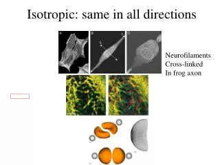
Isotropic: same in all directions Neurofilaments Cross-linked In frog axon
#3- Think of a balloon with stiff meridional bands- networks can stretch more easily along the axis with less stiff ropes. • #4 hoop stress versus axial stress
Buckling & Bending 20 cm 10 cm
Flow Cell 1 cell 2 cell 3 Tension Field Theory Membrane
Inside a Blood Vessel Endothelial cells with Nucleus bulging out Blood flow 10 microns
Cells- fluid or solid? • Micropipet aspiration comparison between ECs and chondrocytes • Comparison between EC cell & nucleus • Stiffness following spreading or adapting to flow. • ECs in flow will minimize force on nucleus • Enucleus = 9Ecytoplasm
Applying global strains to Nucleus1 Round Spread Compression & relaxation done quickly to measure passive props while avoiding adaptation. No hysteresis or plastic behaviour seen in spread cells and nuclei. 1. Caille, N: J. Biomech, 2002 Nucleus
Material properties, not inhomogeneity, explains The non-linear behaviour
Bone Adaptation • Most bones experience 1000’s of loads daily • Bone cells must detect mech signals in situ and adjust bone architecture appropriately. • Sensor cells: Osteocytes; Effector cells: Osteoblasts, osteoclasts • Signalling molecules: PGs, NO • Responses: bone formation/resorption
Bending forces not only cause deformation of osteocytes, but generate pressure gradients that drive fluid flow through the canalicular spaces. Bending causes compressive stress on one side of the bone and tensile stresses on the other. This leads to a pressure gradient in the interstitial fluids that drives fluid flow from regions of compression to tension. Fluid flows through the canaliculae and across the osteocytes, providing nutrients and causing flow-related shear stresses on the cell membranes. The fluid flow also creates an electric potential called a streaming potential
Strain detected by mechanoreceptors or by CAMs. G protein in membrane causes Ca and other 2nd messengers.
osteocytes (Oc) and bone lining cells (BLC) detect mechanical signals and communicate those signals to the bone surface. Soluble mediators, which include • prostaglandins (PGs) and nitric oxide (NO), are released and cause the recruitment and/or differentiation of osteoblasts (Ob) from proliferating and nonproliferating osteoprogenitor cells.
The error function, i.e., the daily loading stimulus (S) • minus the normal loading pattern (F; So), drives bone adaptation. Abnormally low values of the error function cause increased osteoclast activity on bone remodeling surfaces, while abnormally high values cause increased osteoblast activity on bone modeling surfaces
Rats jumping various of numbers of times per day showed that five jumps per day were sufficient to increase bone mass, but increasing numbers of jumps gave diminishing returns with respect to bone mass. These data very closely fit the mathematical relationship proposed in Eq. 1
Load type affects adaptation • Long bones are loaded mostly in bending • Strain @ neutral axis is small, and increases away from axis • Loading that changes the neutral axis, changes bone formation 1 • 1. Turner, CH: J. Orthop. Sci, 1998.
MC3T3-E1 osteoblasts subjected to fluid shear (12dynes/cm2) for 60min undergo dramatic reorganization of the actin • cytoskeleton. A Control cells not subjected to flow have poorly organized stress fibers labeled with Texas red-phalloidin. • B Cells subjected to fluid flow for 60 min develop prominent stress fibers labeled with Texas red-phalloidin that are aligned roughly parallel to each other. C and D Control cells not subjected to fluid shear which have poorly organized stress fibers
Adaptation Cascade • Transduction … Biochemical… transmission….effector cell…..tissue • Ion channels….Ca++,NOS, COX, PGs, G protein….Obs, Ocs…..trabeculae • It is an error driven feedback system • Driven more by infrequent abnormal strains than by normal strains encountered during predominant activity1 • 1. Layton, LE: The success and failure of the adaptive response to functional loading-bearing in averting bone fracture; Bone:13:1992
Resonant Stimuli for Bone • Loading frequencies near 20 Hz • Vibration 1 • Error Driven • 1. Rubin, C.
Mechano - regulation • Growth, proliferation, protein synthesis, gene expression, homeostasis. • Transduction process- how? • Single cells do not provide enough material. • MTC can perturb ~ 30,000 cells and is limited. • MTS is more versatile- more cells, longer periods, varied waveforms..
Markov Chains • A dynamic model describing random movement over time of some activity • Future state can be predicted based on current probability and the transition matrix
Sliding Filament Model Ratchet For A-M, vo = 0.5 um/s
Harmonic motion (undamped) Gel motion follows simple rules Model will predict dynamic and Static equilibrium. Natural Frequency
Transition Probabilities Today’s Game Outcome Need a P for Today’s game Tomorrow’s Game Outcome
Good Bad Good 3/4 1/2 Bad 1/4 1/2 Sum 1 1 Grades Transition Matrix This Semester Grade Tendencies To predict future: Start with now: What are the grade probabilities for this semester? Next Semester
Markov Chain Intial Probability Set independently
Computing Markov Chains % A is the transition probability A= [.75 .5 .25 .5] % P is starting Probability P=[.1 .9] for i = 1:20 P(:,i+1)=A*P(:,i) end