Review of Basic Statistical Concepts
Review of Basic Statistical Concepts. Farideh Dehkordi-Vakil. Inferential Statistics. Introduction to Inference The purpose of inference is to draw conclusions from data.

Review of Basic Statistical Concepts
E N D
Presentation Transcript
Review of Basic Statistical Concepts Farideh Dehkordi-Vakil
Inferential Statistics • Introduction to Inference • The purpose of inference is to draw conclusions from data. • Conclusions take into account the natural variability in the data, therefore formal inference relies on probability to describe chance variation. • We will go over the two most prominent types of formal statistical inference • Confidence Intervals for estimating the value of a population parameter. • Tests of significance which asses the evidence for a claim. • Both types of inference are based on the sampling distribution of statistics.
Inferential Statistics • Since both methods of formal inference are based on sampling distributions, they require probability model for the data. • The model is most secure and inference is most reliable when the data are produced by a properly randomized design. • When we use statistical inference we assume that the data come from a randomly selected sample or a randomized experiment.
Inferential Statistics • A market research firm interviews a random sample of 2500 adults. Results: 66% find shopping for cloths frustrating and time consuming. • That is the truth about the 2500 people in the sample. • What is the truth about almost 210 million American adults who make up the population? • Since the sample was chosen at random, it is reasonable to think that these 2500 people represent the entire population pretty well.
Inferential Statistics • Therefore, the market researchers turn the fact that 66% of sample find shopping frustrating into an estimate that about 66% of all adults feel this way. • Using a fact about a sample to estimate the truth about the whole population is called statistical inference. • To think about inference, we must keep straight whether a number describes a sample or a population.
Inferential Statistics • Parameters and Statistics • A parameter is a number that describes the population. • A parameter is a fixed number, but in practice we do not know its value. • A statistic is a number that describes a sample. • The value of a statistic is known when we have taken a sample, but it can change from sample to sample. • We often use statistic to estimate an unknown parameter.
Inferential Statistics • Changing consumer attitudes towards shopping are of great interest to retailers and makers of consumer goods. • One trend of concern to marketers is that fewer people enjoy shopping than in the past. • A market research firm conducts an annual survey of consumer attitudes. • The population is all Us residents aged 18 and over.
Example:Consumer attitude towards shopping • A recent survey asked a nationwide random sample of 2500 adults if they agreed or disagreed that “ I like buying new cloths, but shopping is often frustrating and time consuming.” • Of the respondents, 1650 said they agreed. • The proportion of the sample who agreed that cloths shopping is often frustrating is:
Example:Consumer attitude towards shopping • The number = .66 is a statistic. • The corresponding parameter is the proportion (call it P) of all adult U.S. residents who would have said “agree” if asked the same question. • We don’t know the value of parameterP, so we use as its estimate.
Inferential Statistics • If the marketing firm took a second random sample of 2500 adults, the new sample would have different people in it. • It is almost certain that there would not be exactly 1650 positive responses. • That is, the value of will vary from sample to sample. • Random samples eliminate bias from the act of choosing a sample, but they can still be wrong because of the variability that results when we choose at random.
Inferential Statistics • The first advantage of choosing at random is that it eliminates bias. • The second advantage is that if we take lots of random samples of the same size from the same population, the variation from sample to sample will follow a predictable pattern. • All statistical inference is based on one idea: to see how trustworthy a procedure is, ask what would happen if we repeated it many times.
Inferential Statistics • Suppose that exactly 60% of adults find shopping for cloths frustrating and time consuming. • That is, the truth about the population is that P = 0.6. • What if we select an SRS of size 100 from this population and use the sample proportion to estimate the unknown value of the population proportion P?
Inferential Statistics • To answer this question: • Take a large number of samples of size 100 from this population. • Calculate the sample proportion for each sample. • Make a histogram of the values of . • Examine the distribution displayed in the histogram for shape, center, and spread, ass well as outliers or other deviations.
Inferential Statistics • The result of many SRS have a regular pattern. • Here we draw 1000 SRS of size 100 from the same population. • The histogram shows the distribution of the 1000 sample proportions
Inferential Statistics • Sampling Distribution • The sampling distribution of a statistic is the distribution of values taken by the statistic in all possible samples of the same size from the same population.
Example:Mean income of American households • What is the mean income of households in the United States? • The Bureau of Labor Statistics contacted a random sample of 55,000 households in March 2001 for the current population survey. • The mean income of the 55,000 households for the year 2000 was • $57,045 is a statistic that describes the CPS sample households.
Example:Mean income of American households • We use it to estimate an unknown parameter, the mean income of all 106 million American households. • We know that would take several different values if the Bureau of Labor Statistics had taken several samples in March 2001. • We also know that this sampling variability follows a regular pattern that can tell us how accurate the sample result is likely to be. • That pattern obeys the laws of probability.
Normal Density Curve • These density curves, called normal curves, are • Symmetric • Single peaked • Bell shaped • Normal curves describe normal distributions.
Normal Density Curve • The exact density curve for a particular normal distribution is described by giving its mean and its standard deviation . • The mean is located at the center of the symmetric curve and it is the same as the median. • The standard deviation controls the spread of a normal curve.
The 68-95-99.7 Rule • Although there are many normal curve, They all have common properties. In particular, all Normal distributions obey the following rule. • In a normal distribution with mean and standard deviation : • 68% of the observations fall within of the mean . • 95% of the observations fall within 2 of . • 99.7% of the observations fall within 3 of .
Inferential Statistics • Standardizing and z-score • If x is an observation that has mean and standard deviation , the standardized value of x is • A standardized value is often called z-score.
Standard Normal Distribution • The standard Normal distribution is the Normal distribution N(0, 1) with mean = 0 and standard deviation =1.
Standard Normal Distribution • If a variable x has any normal distribution N(, ) with mean and standard deviation , then the standardized variable has the standard Normal distribution.
The Standard Normal Table • Table A is a table area under the standard Normal curve. The table entry for each value z is the area under the curve to the left of z.
The Standard Normal Table • What the area under the standard normal curve to the right of z = - 2.15? • Compact notation: z < -2.15 • P = 1 - .0158 =.9842
The Standard Normal Table • What is the area under the standard normal curve between z = 0 and z = 2.3? • Compact notation: 0 < z < 2.3 • P = .9893 - .5 =.4893
Example:Annual rate of return on stock indexes The annual rate of return on stock indexes (which combine many individual stocks) is approximately Normal. Since 1954, the S&P 500 stock index has had a mean yearly return of about 12%, with standard deviation of 16.5%. Take this Normal distribution to be the distribution of yearly returns over a long period. The market is down for the year if the return on the index is less than zero. In what proportion of years is the market down?
Example:Annual rate of return on stock indexes • State the problem • Call the annual rate of return for S& P 500-stocks Index x. The variable x has the N(12, 16.5) distribution. We want the proportion of years with X < 0. • Standardize • Subtract the mean, then divide by the standard deviation, to turn x into a standard Normal z:
Example:Annual rate of return on stock indexes • Draw a picture to show the standard normal curve with the area of interest shaded. • Use the table • The proportion of observations less than - 0.73 is .2327. • The market is down on an annual basis about 23.27% of the time.
Example:Annual rate of return on stock indexes • What percent of years have annual return between 12% and 50%? • State the problem • Standardize
Example:Annual rate of return on stock indexes • Draw a picture. • Use table. • The area between 0 and 2.30 is the area below 2.30 minus the area below 0. 0.9893- .50 = .4893
Estimating with Confidence • Community banks are banks with less than a billion dollars of assets. There are approximately 7500 such banks in the United States. In many studies of the industry these banks are considered separately from banks that have more than a billion dollars of assets. The latter banks are called “large institutions.” The community bankers Council of the American bankers Association (ABA) conducts an annual survey of community banks. For the 110 banks that make up the sample in a recent survey, the mean assets are = 220 (in millions of dollars). What can we say about , the mean assets of all community banks?
Estimating with Confidence • The sample mean is the natural estimator of the unknown population mean . • We know that • is an unbiased estimator of . • The law of large numbers says that the sample mean must approach the population mean as the size of the sample grows. • Therefore, the value = 220 appears to be a reasonable estimate of the mean assets for all community banks. • But, how reliable is this estimate?
Estimating with Confidence • An estimate without an indication of its variability is of limited value. • Questions about variation of an estimator is answered by looking at the spread of its sampling distribution. • According to Central Limit theorem: • If the entire population of community bank assets has mean and standard deviation , then in repeated samples of size 110 the sample mean approximately follows the N(, 110) distribution
Estimating with Confidence • Suppose that the true standard deviation is equal to the sample standard deviation s = 161. • This is not realistic, although it will give reasonably accurate results for samples as large as 100. Later on we will learn how to proceed when is not known. • Therefore, by Central Limit theorem. In repeated sampling the sample mean is approximately normal, centered at the unknown population mean ,with standard deviation
Confidence Interval • A level C confidence interval for a parameter has two parts: • An interval calculated from the data, usually of the form Estimate margin of error • A confidence Level C, which gives the probability that the interval will capture the true parameter value in repeated samples.
Confidence Interval • We use the sampling distribution of the sample mean to construct a level C confidence interval for the mean of a population. • We assume that data are a SRS of size n. • The sampling distribution is exactly N( ) when the population has the N(, ) distribution. • The central Limit theorem says that this same sampling distribution is approximately correct for large samples whenever the population mean and standard deviation are and .
Confidence Interval for a Population Mean • Choose a SRS of size n from a population having unknown mean and known standard deviation . A level C confidence interval for is Here z* is the critical value with area C between –z* and z* under the standard Normal curve. The quantity is the margin of error. The interval is exact when the population distribution is normal and is approximately correct when n is large in other cases.
Example: Banks’ loan –to-deposit ration • The ABA survey of community banks also asked about the loan-to-deposit ratio (LTDR), a bank’s total loans as a percent of its total deposits. The mean LTDR for the 110 banks in the sample is and the standard deviation is s = 12.3. This sample is sufficiently large for us to use s as the population here. Find a 95% confidence interval for the mean LTDR for community banks.
Tests of Significance • Confidence intervals are appropriate when our goal is to estimate a population parameter. • The second type of inference is directed at assessing the evidence provided by the data in favor of some claim about the population. • A significance test is a formal procedure for comparing observed data with a hypothesis whose truth we want to assess. • The hypothesis is a statement about the parameters in a population or model. • The results of a test are expressed in terms of a probability that measures how well the data and the hypothesis agree.
Example: Bank’s net income • The community bank survey described in previously also asked about net income and reported the percent change in net income between the first half of last year and the first half of this year. The mean change for the 110 banks in the sample is Because the sample size is large, we are willing to use the sample standard deviation s = 26.4% as if it were the population standard deviation . The large sample size also makes it reasonable to assume that is approximately normal.
Example: Bank’s net income • Is the 8.1% mean increase in a sample good evidence that the net income for all banks has changed? • The sample result might happen just by chance even if the true mean change for all banks is = 0%. • To answer this question we asks another • Suppose that the truth about the population is that = 0% (this is our hypothesis) • What is the probability of observing a sample mean at least as far from zero as 8.1%?
Example: Bank’s net income • The answer is: • Because this probability is so small, we see that the sample mean is incompatible with a population mean of = 0. • We conclude that the income of community banks has changed since last year.
Example: Bank’s net income • The fact that the calculated probability is very small leads us to conclude that the average percent change in income is not in fact zero. Here is why. • If the true mean is = 0, we would see a sample mean as far away as 8.1% only six times per 10000 samples. • So there are only two possibilities: • = 0 and we have observed something very unusual, or • is not zero but has some other value that makes the observed data more probable
Example: Bank’s net income • We calculated a probability taking the first of these choices as true ( = 0 ). That probability guides our final choice. • If the probability is very small, the data don’t fit the first possibility and we conclude that the mean is not in fact zero.
Tests of Significance: Formal details • The first step in a test of significance is to state a claim that we will try to find evidence against. • Null Hypothesis H0 • The statement being tested in a test of significance is called the null hypothesis. • The test of significance is designed to assess the strength of the evidence against the null hypothesis. • Usually the null hypothesis is a statement of “no effect” or “no difference.” We abbreviate “null hypothesis” as H0.
Tests of Significance: Formal details • A null hypothesis is a statement about a population, expressed in terms of some parameter or parameters. • The null hypothesis in our bank survey example is H0 : = 0 • It is convenient also to give a name to the statement we hope or suspect is true instead of H0. • This is called the alternative hypothesis and is abbreviated as Ha. • In our bank survey example the alternative hypothesis states that the percent change in net income is not zero. We write this as Ha : 0